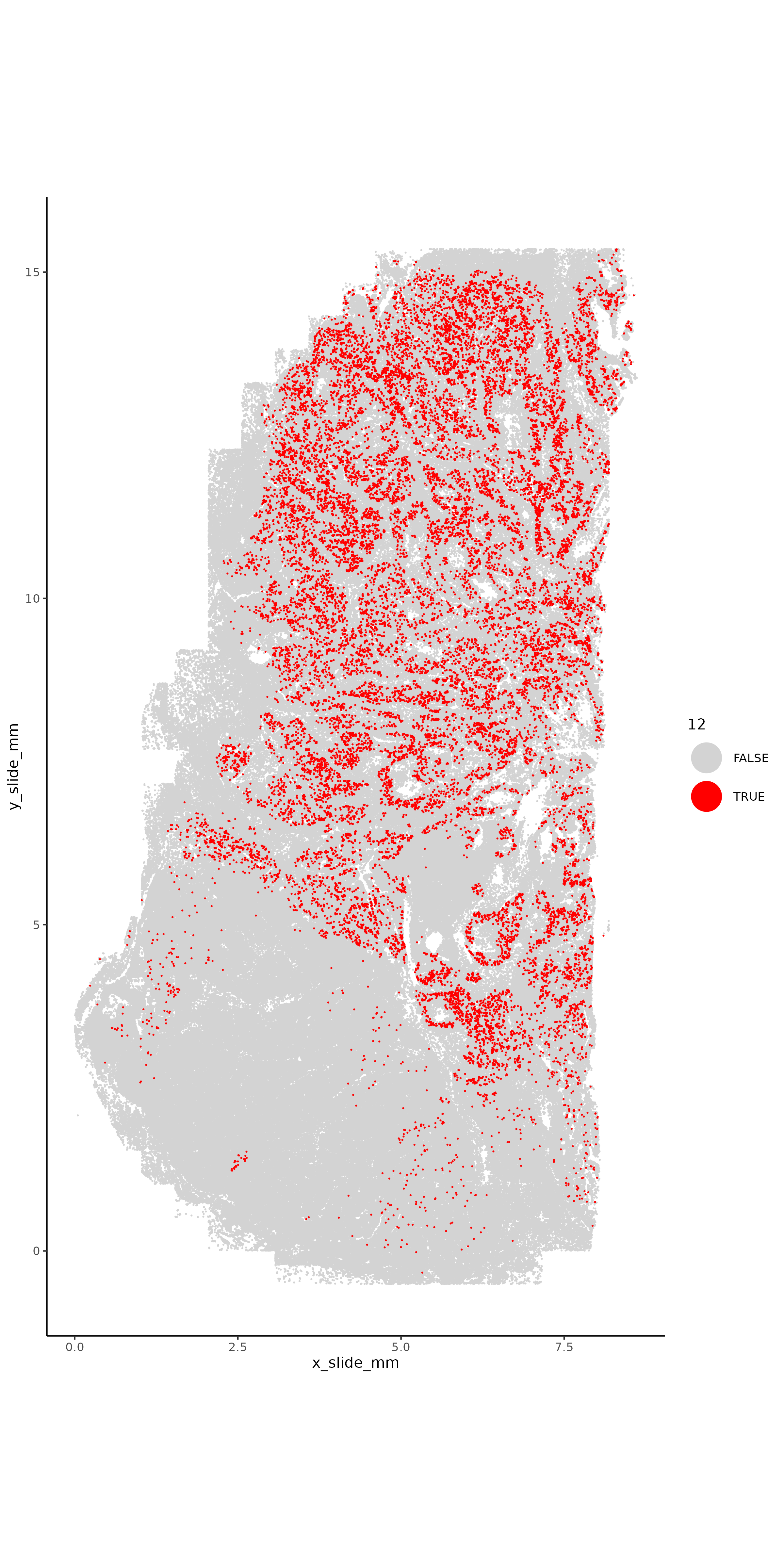
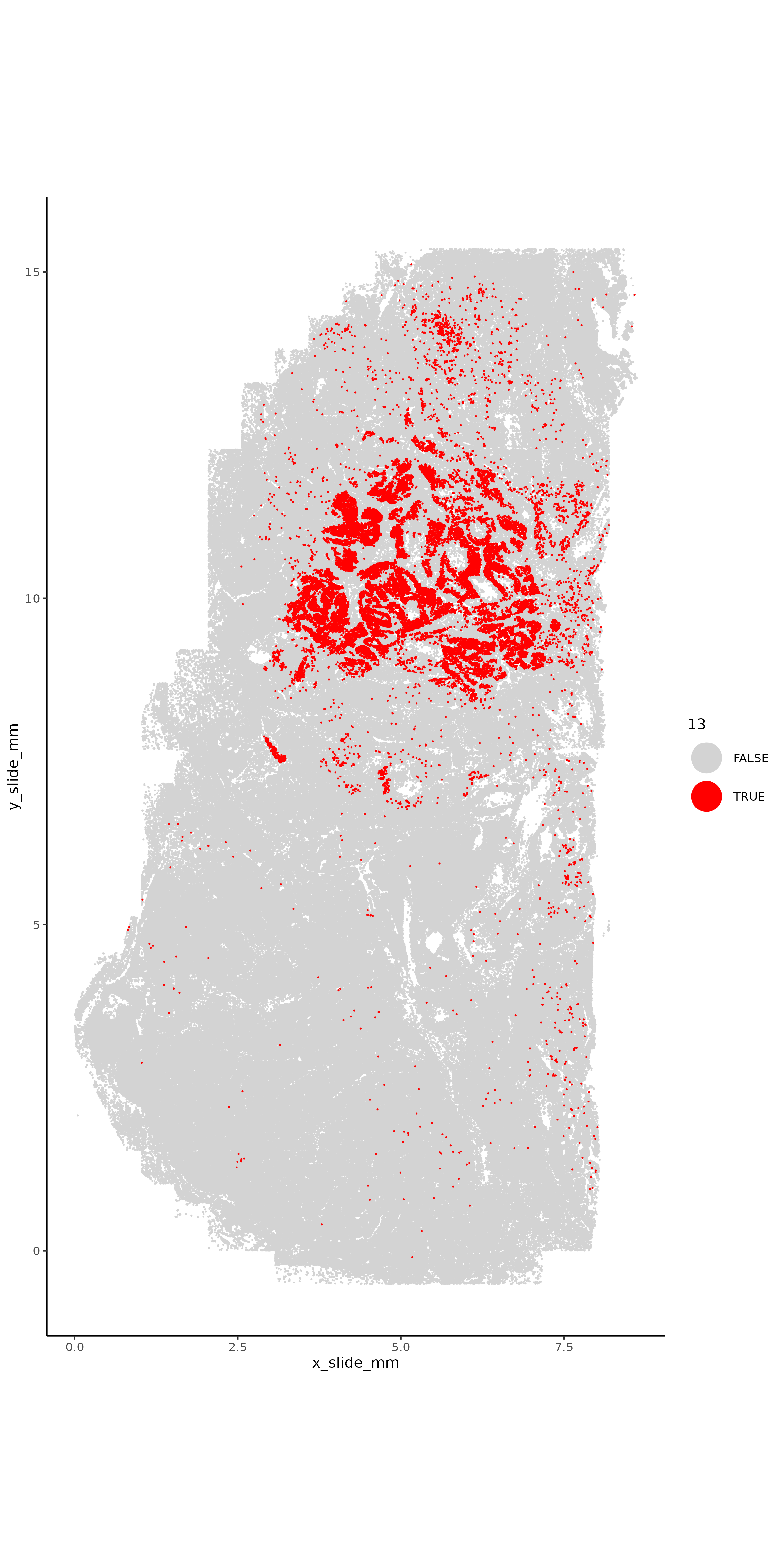
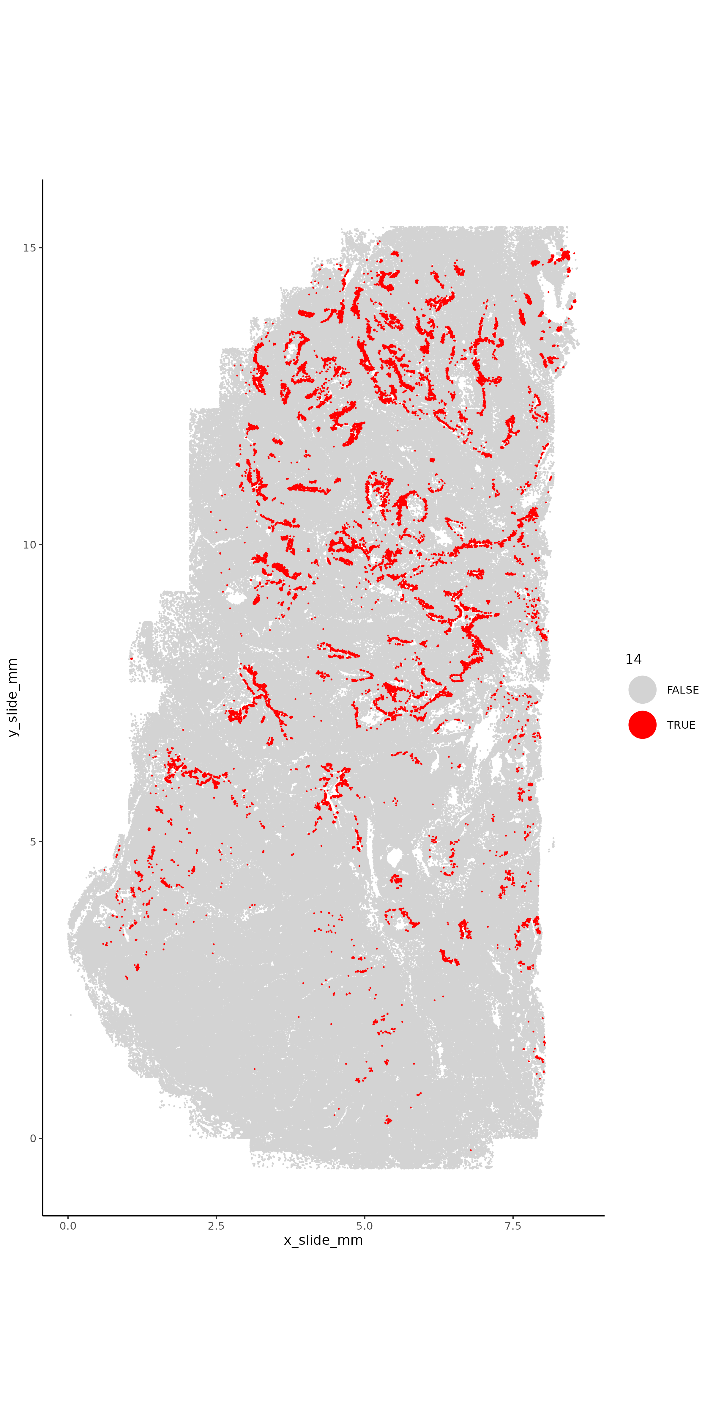
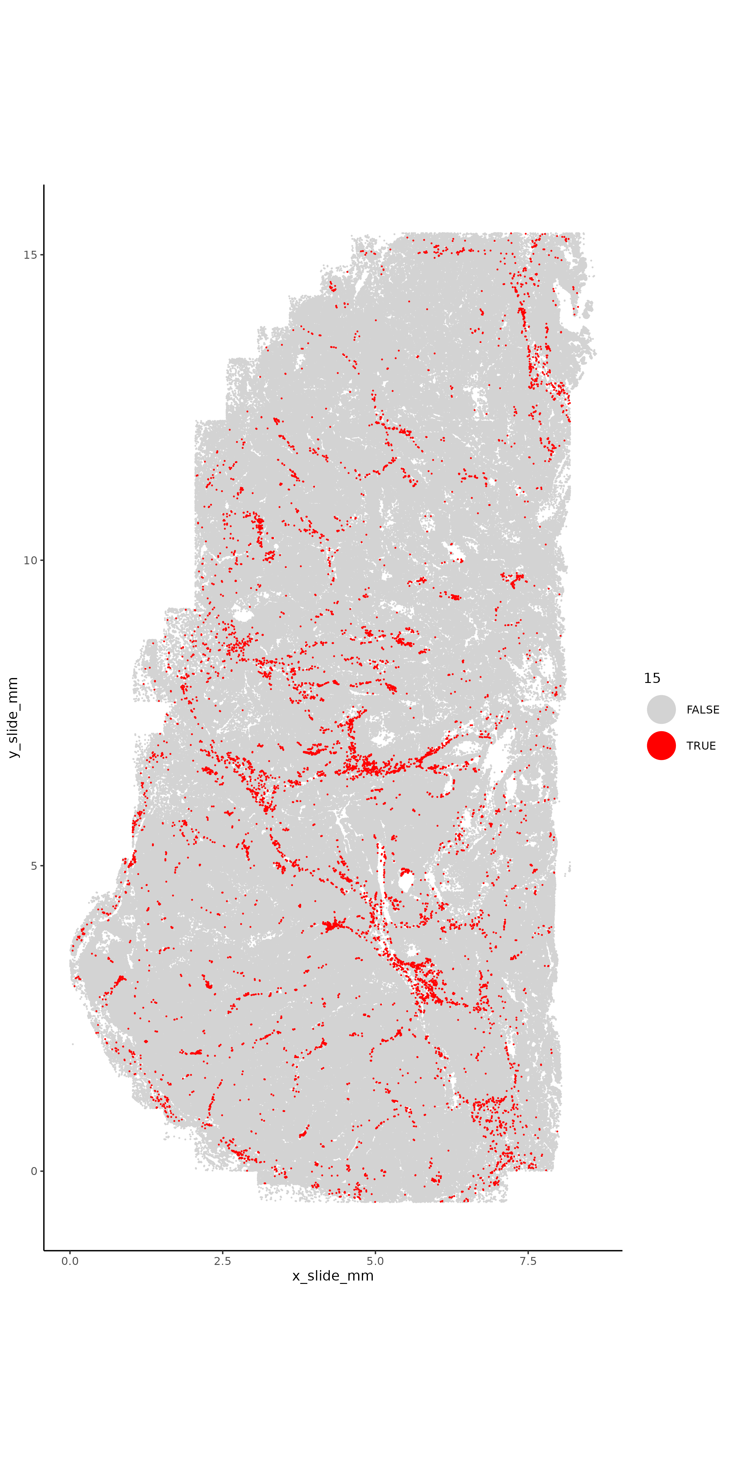
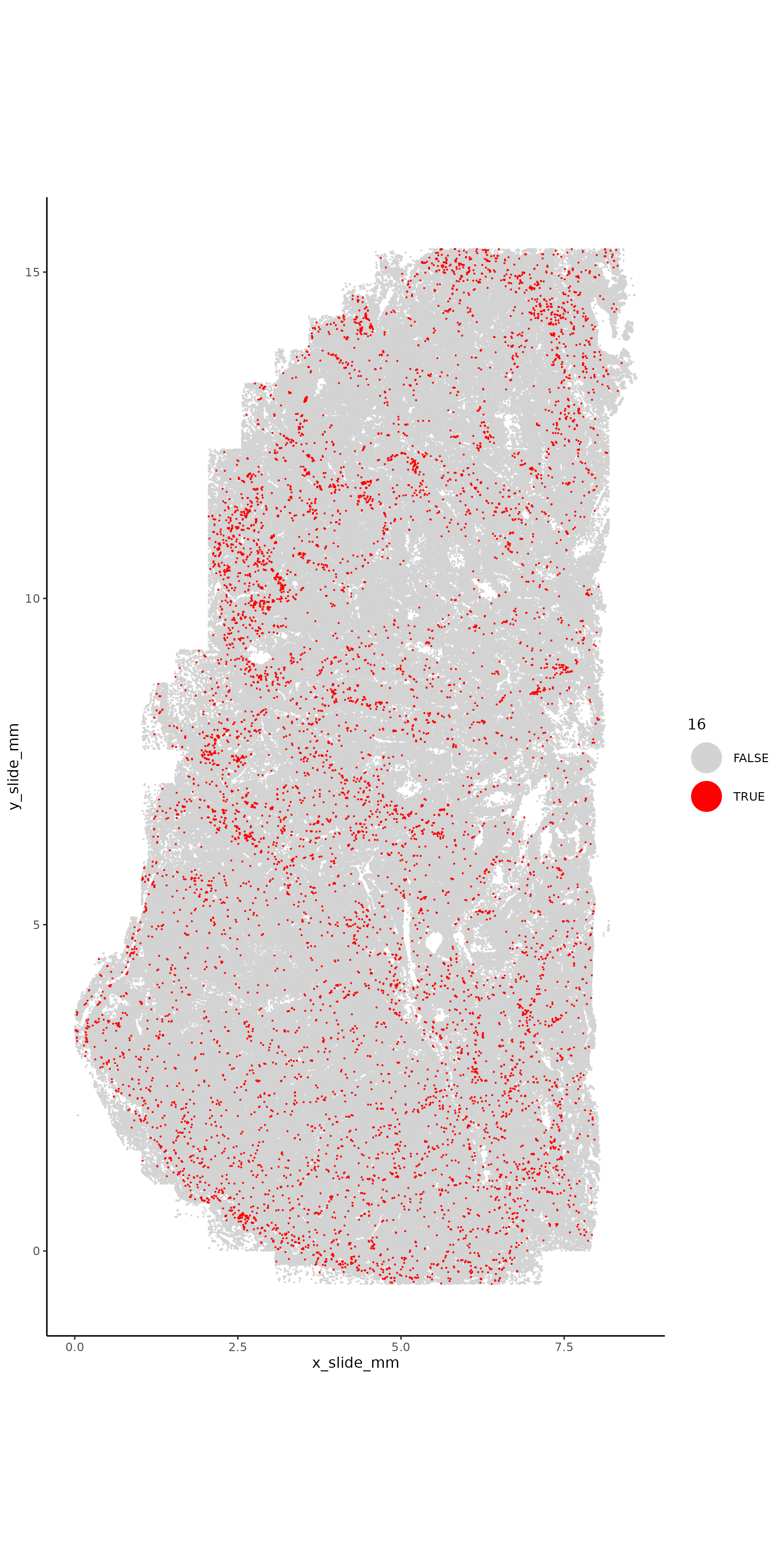
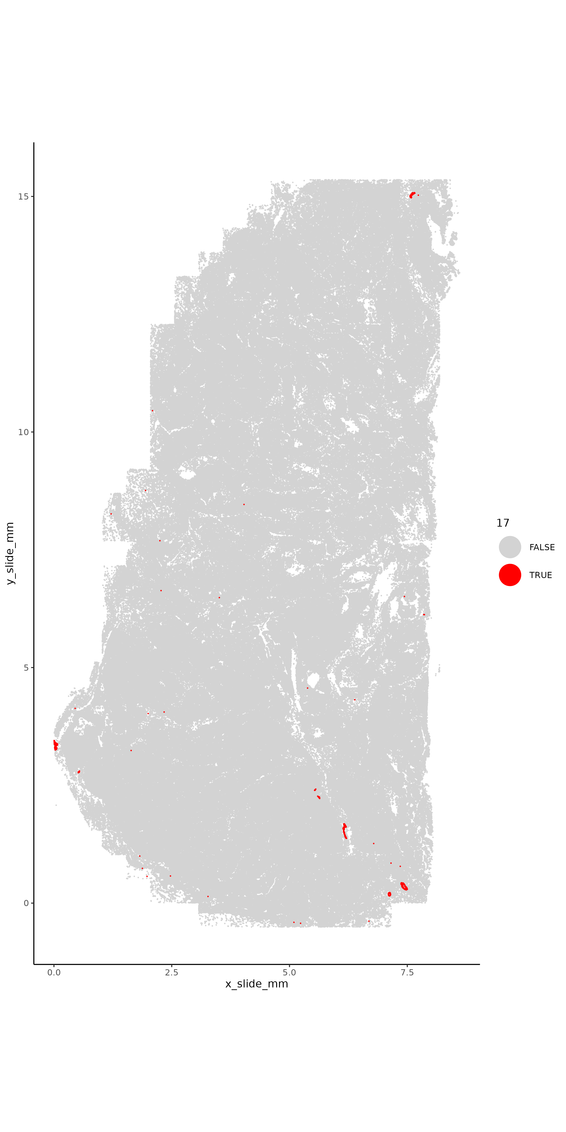
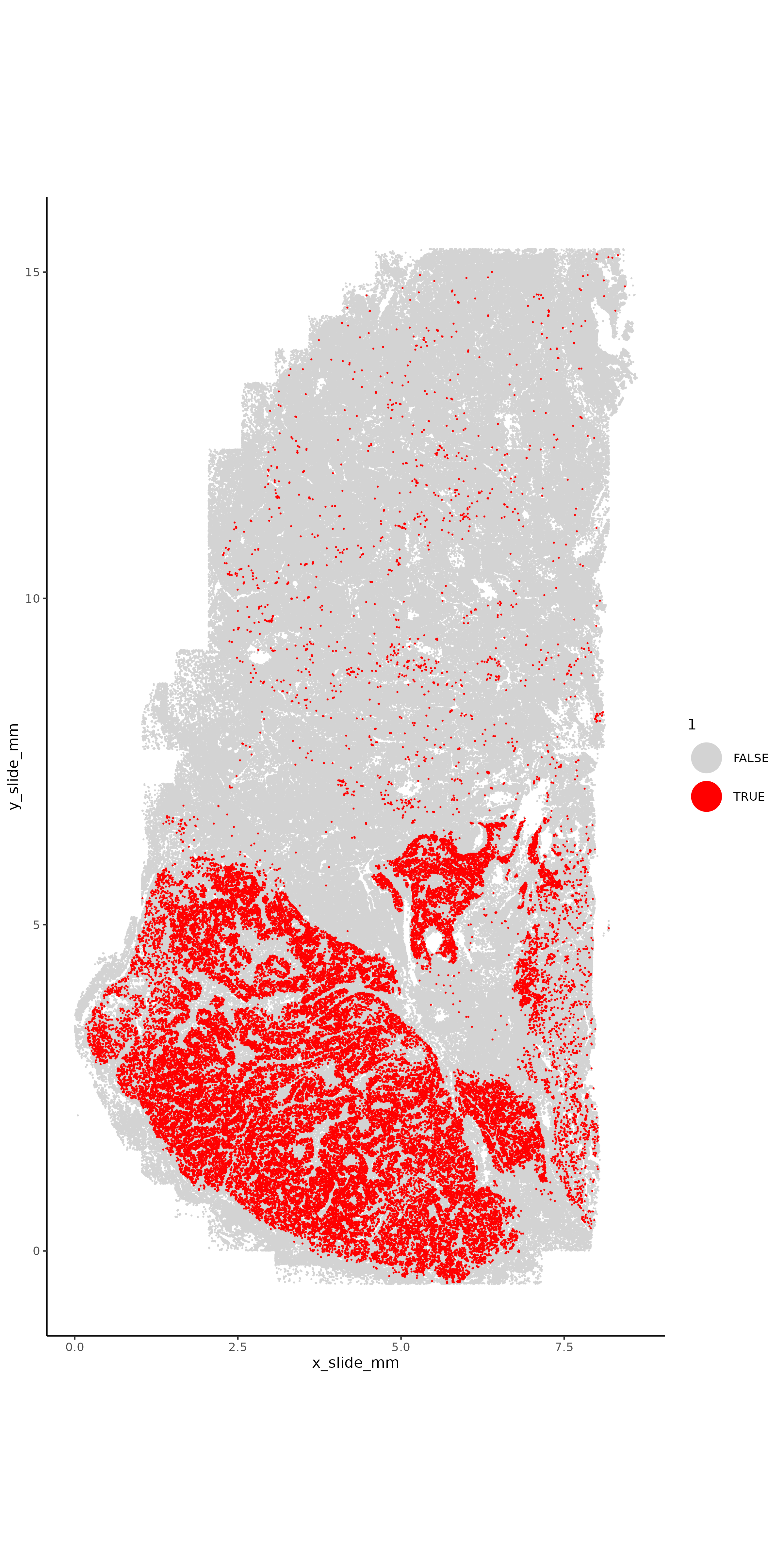
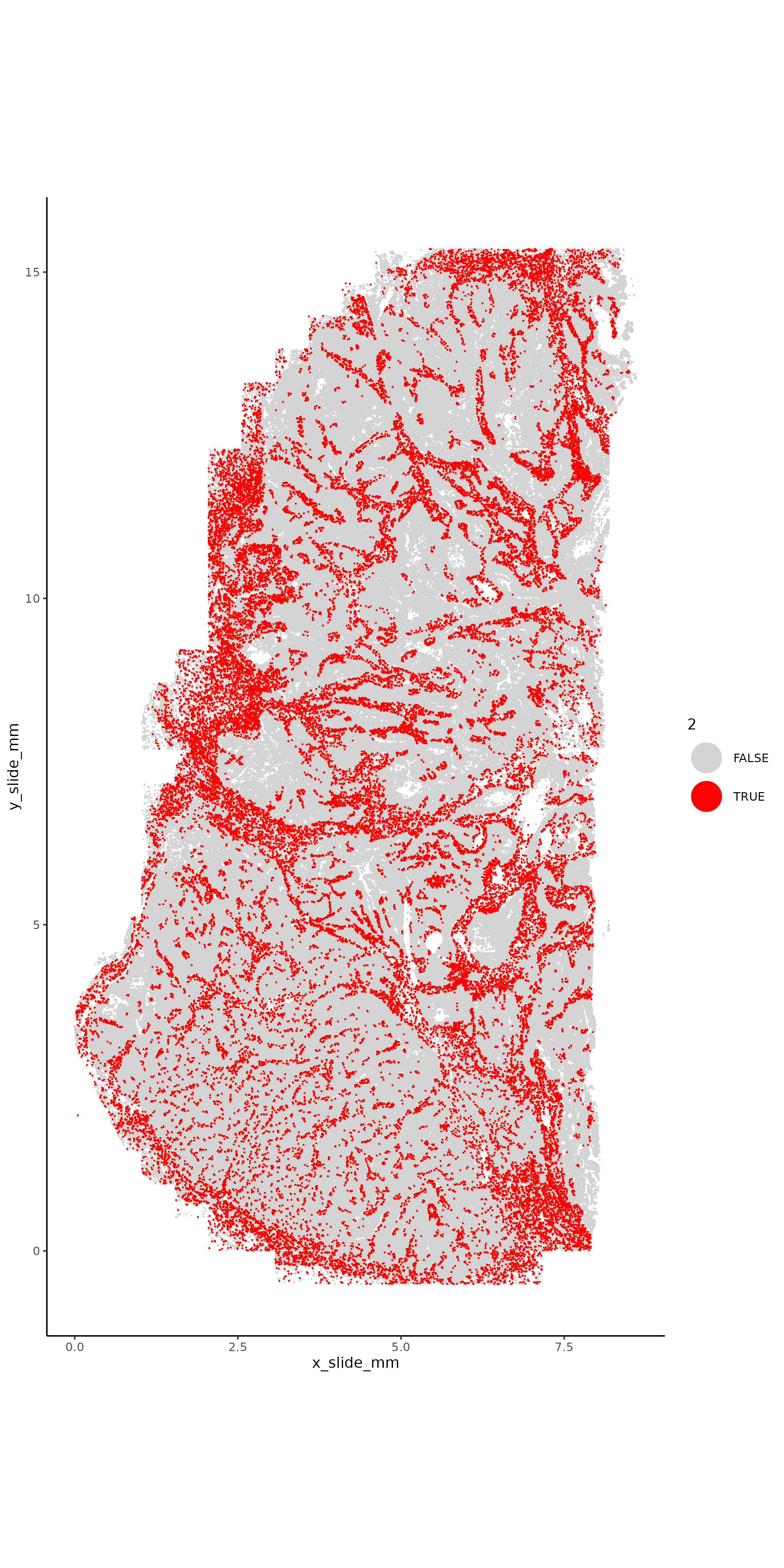
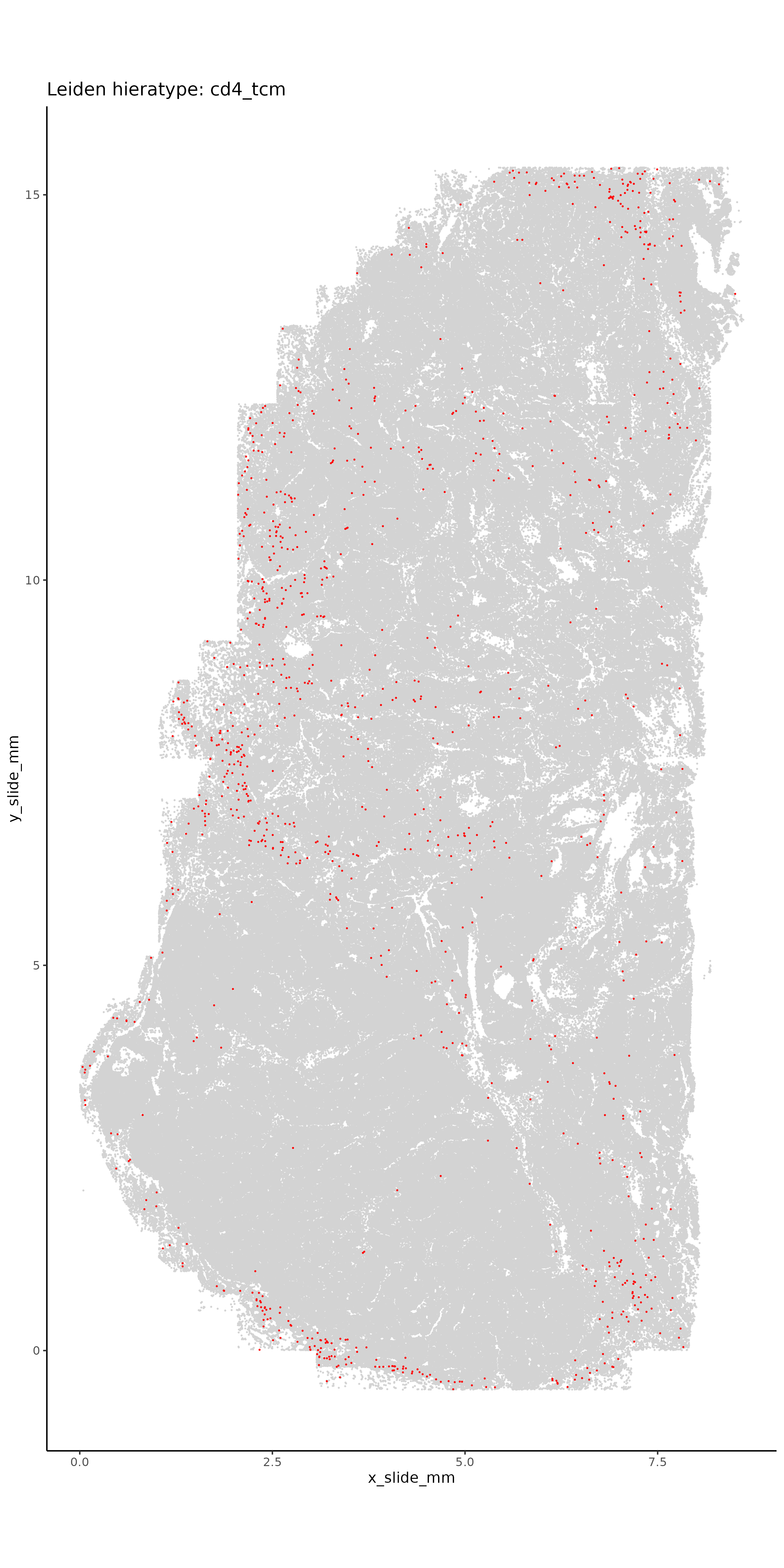
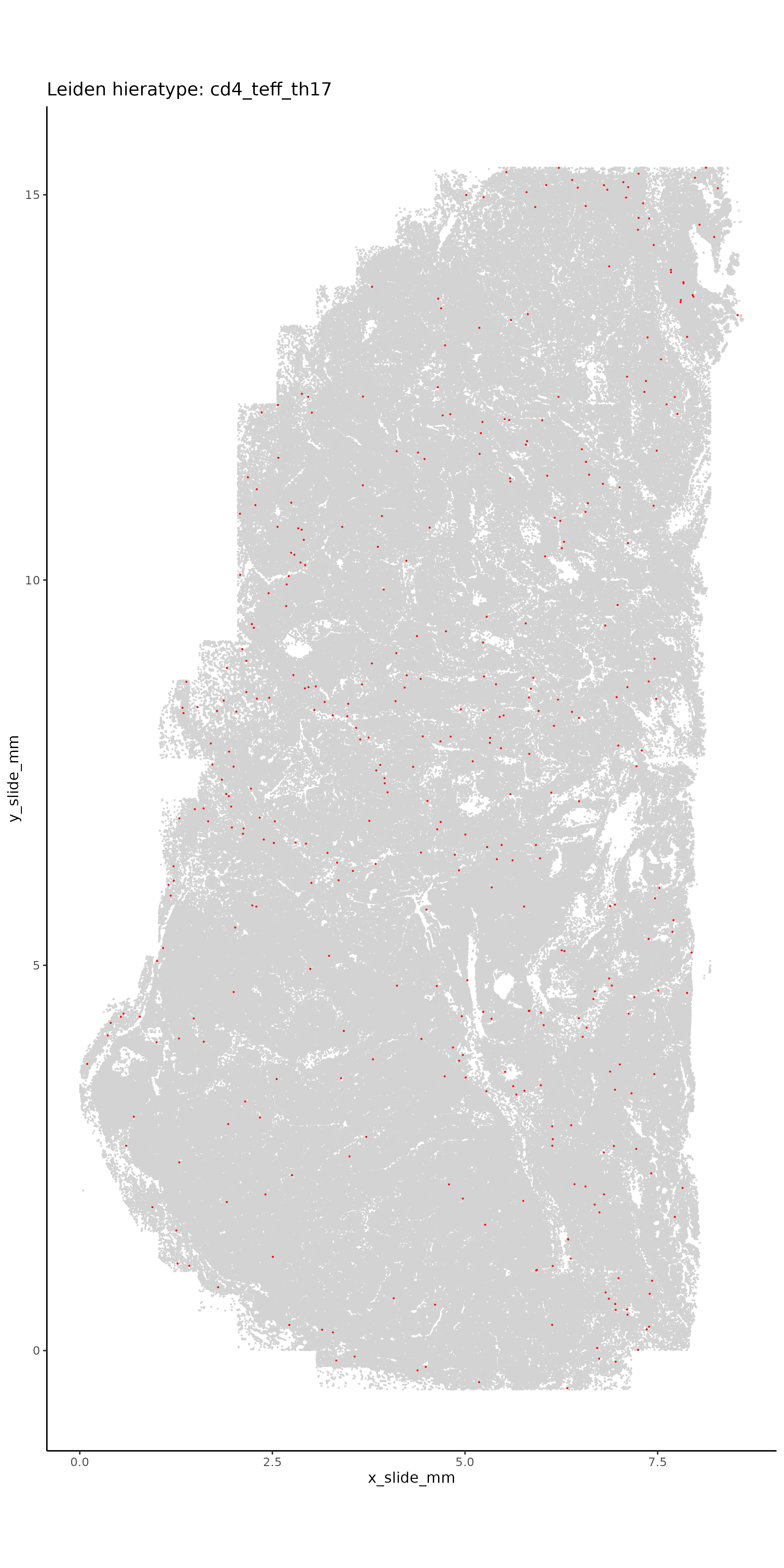
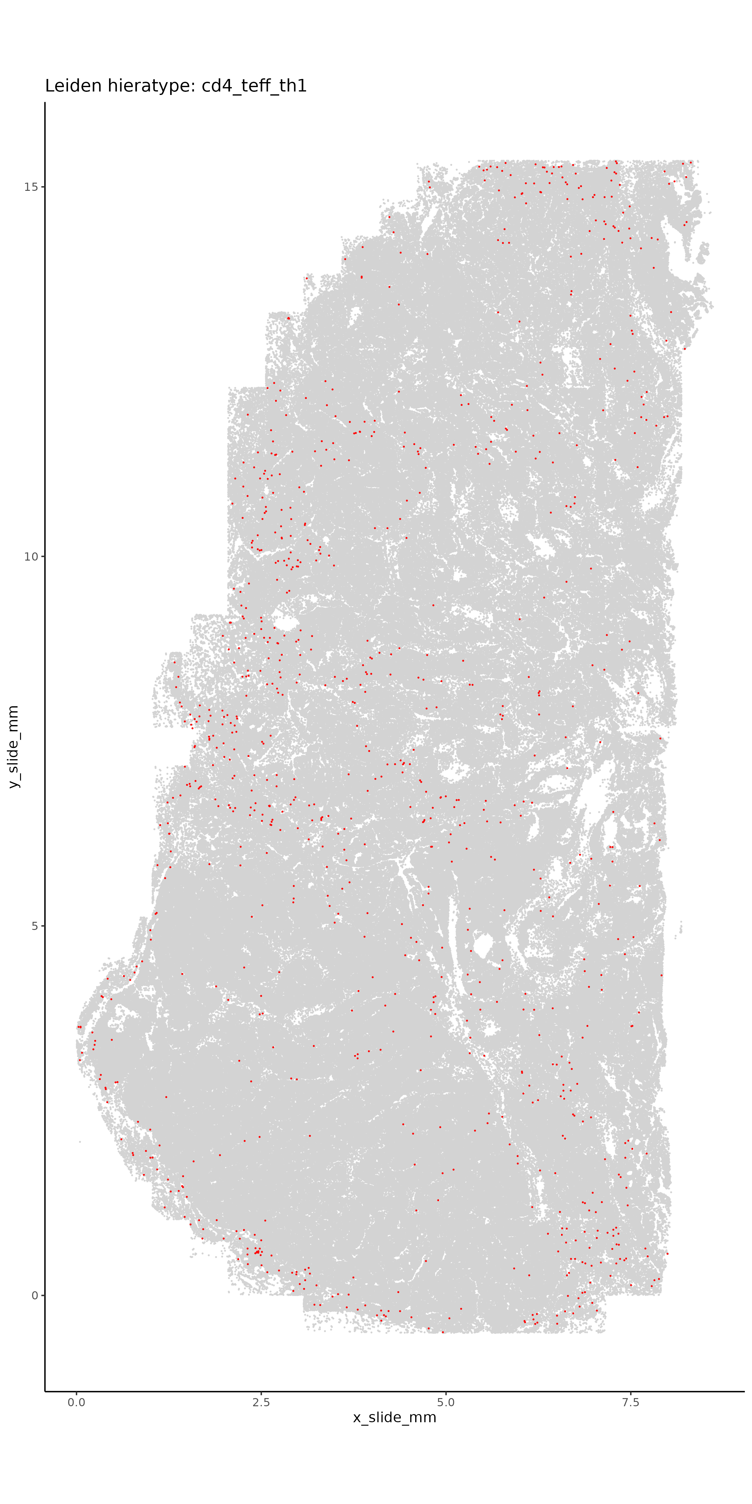
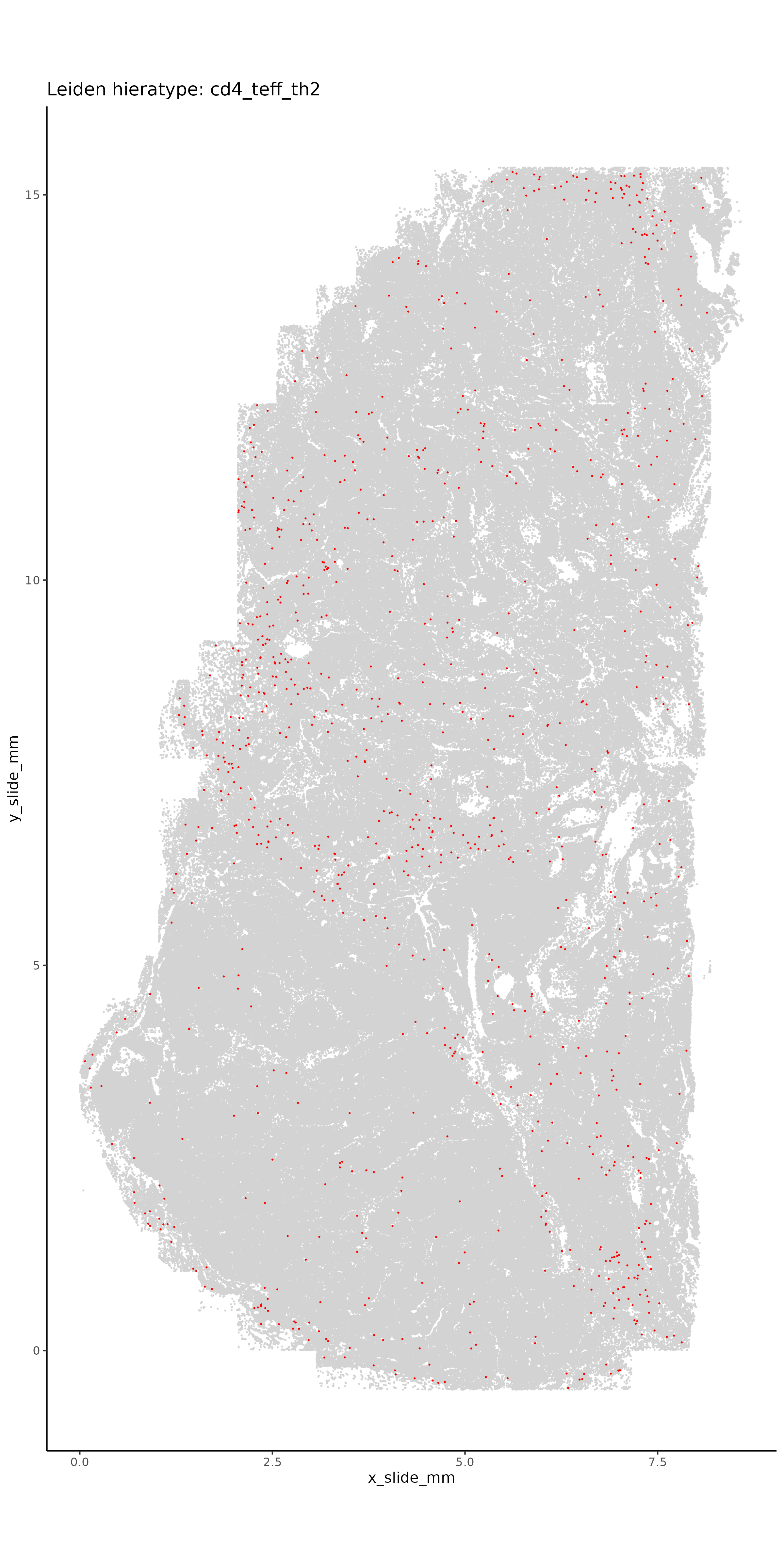
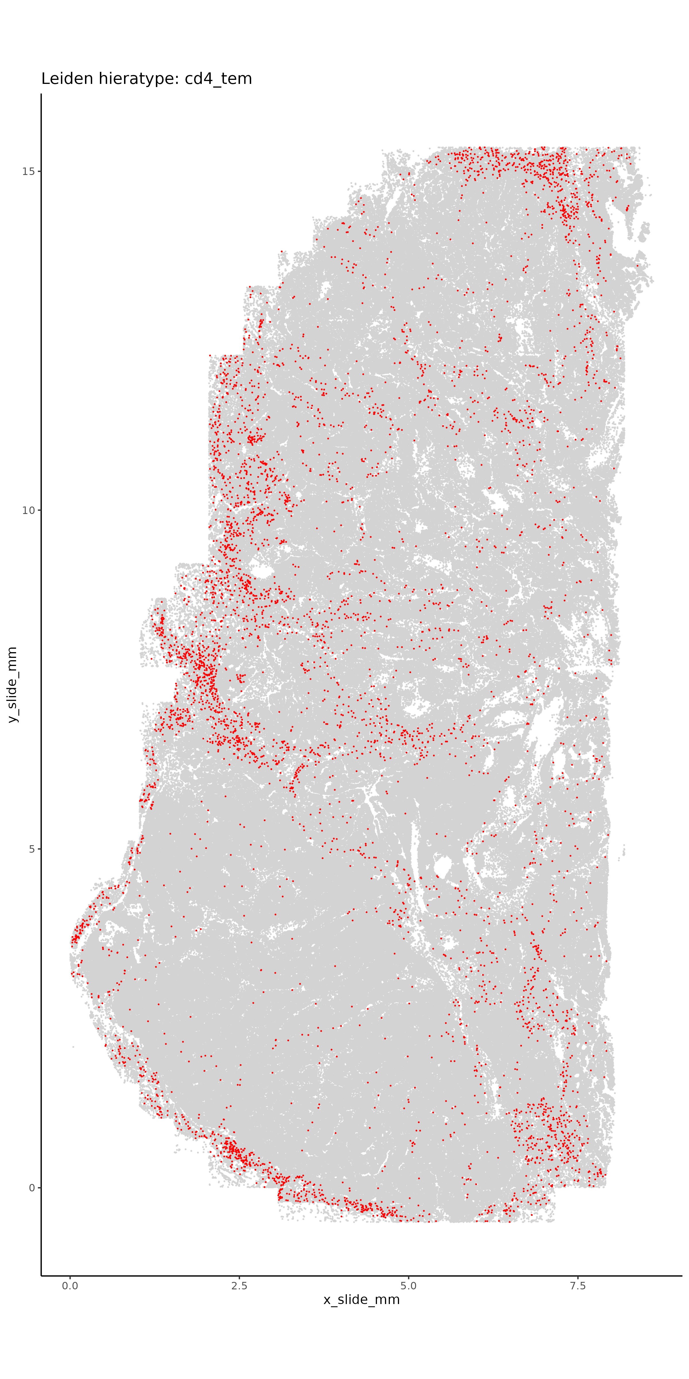
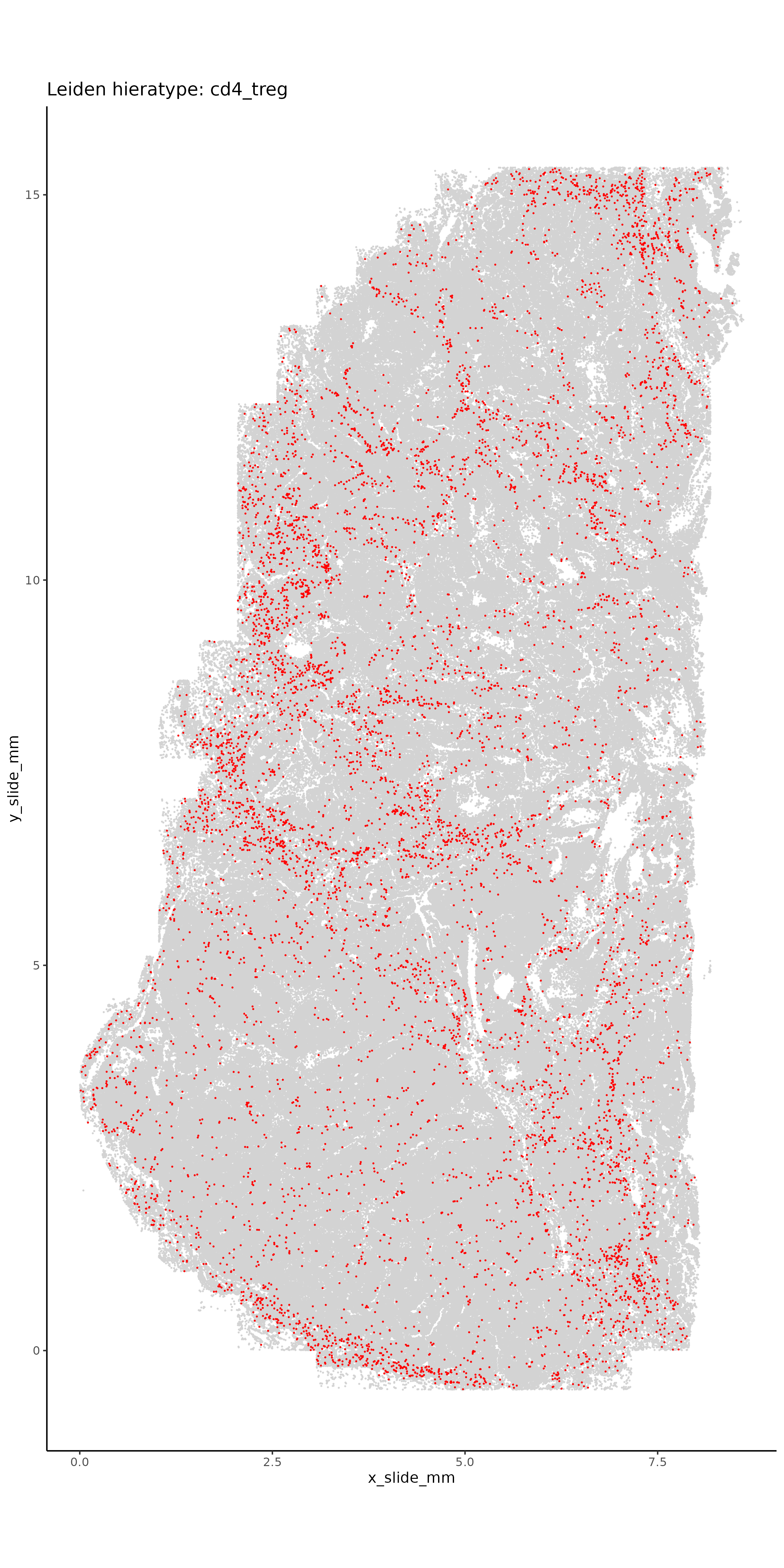
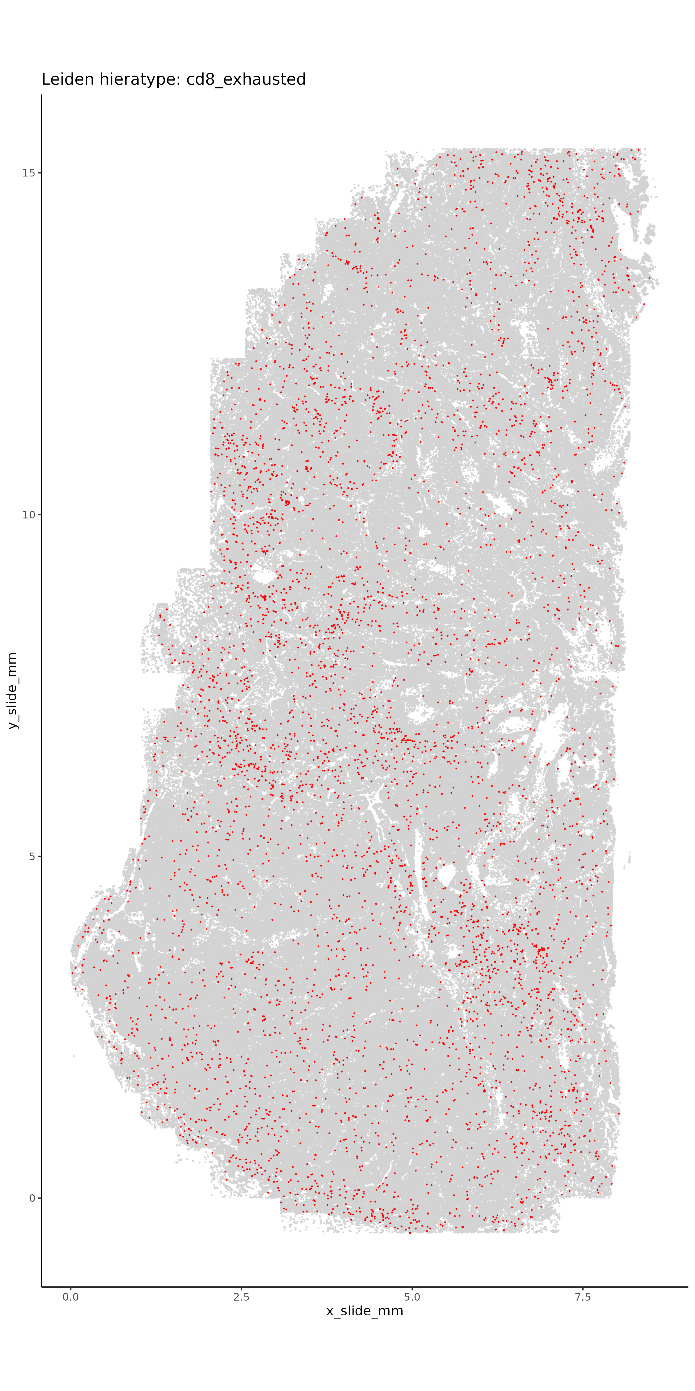
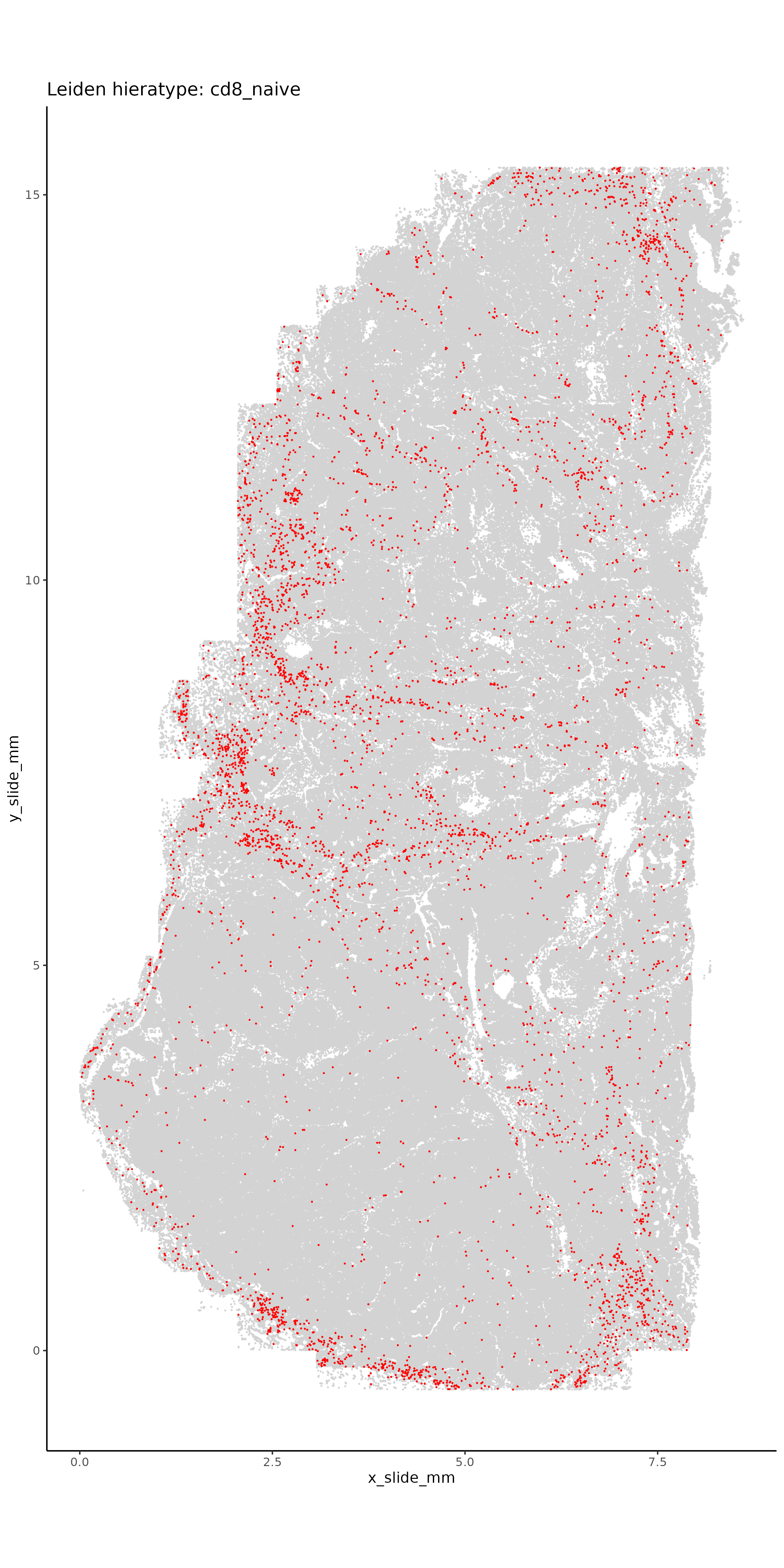
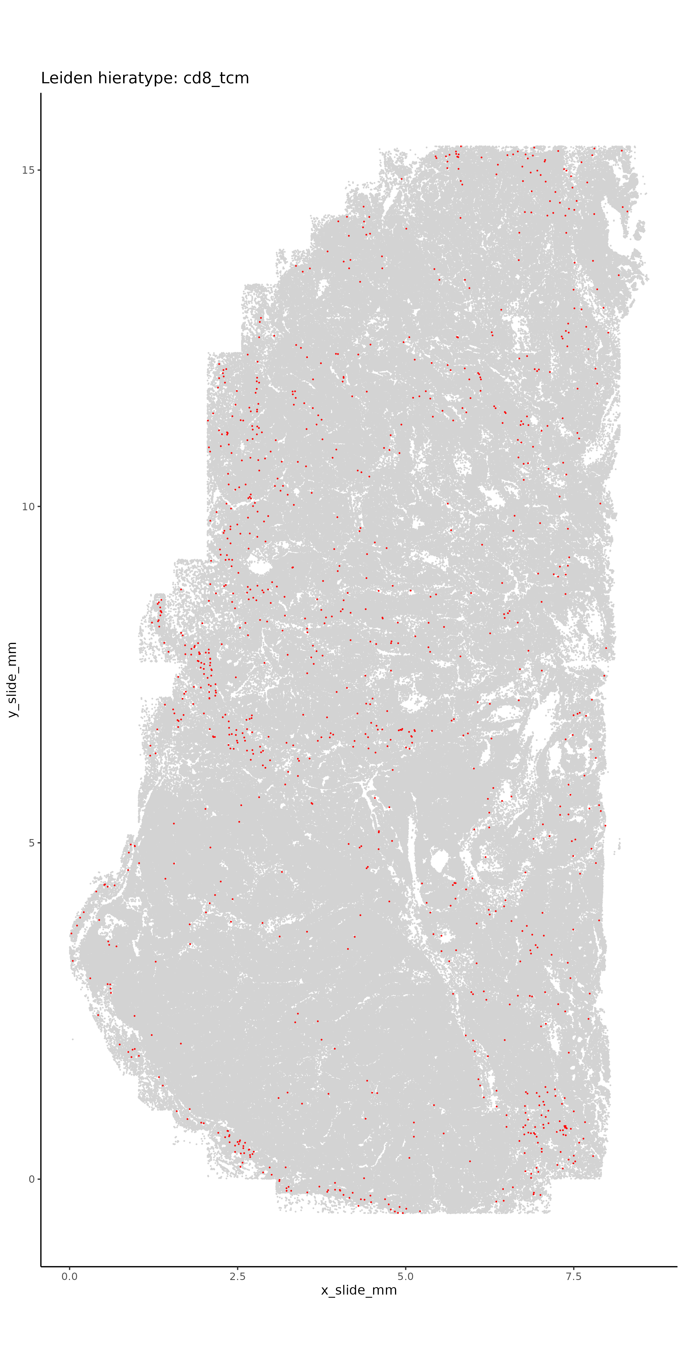
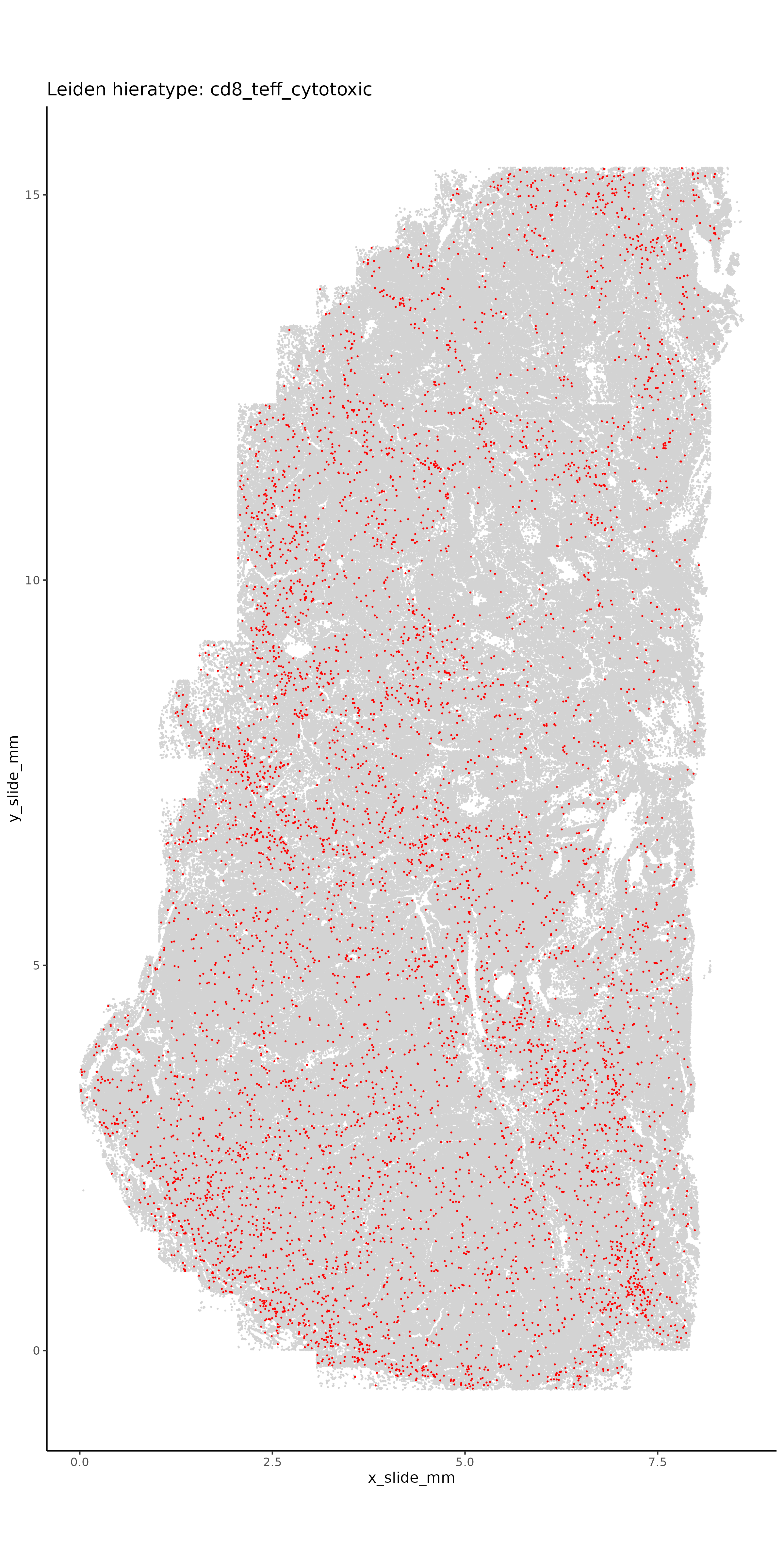
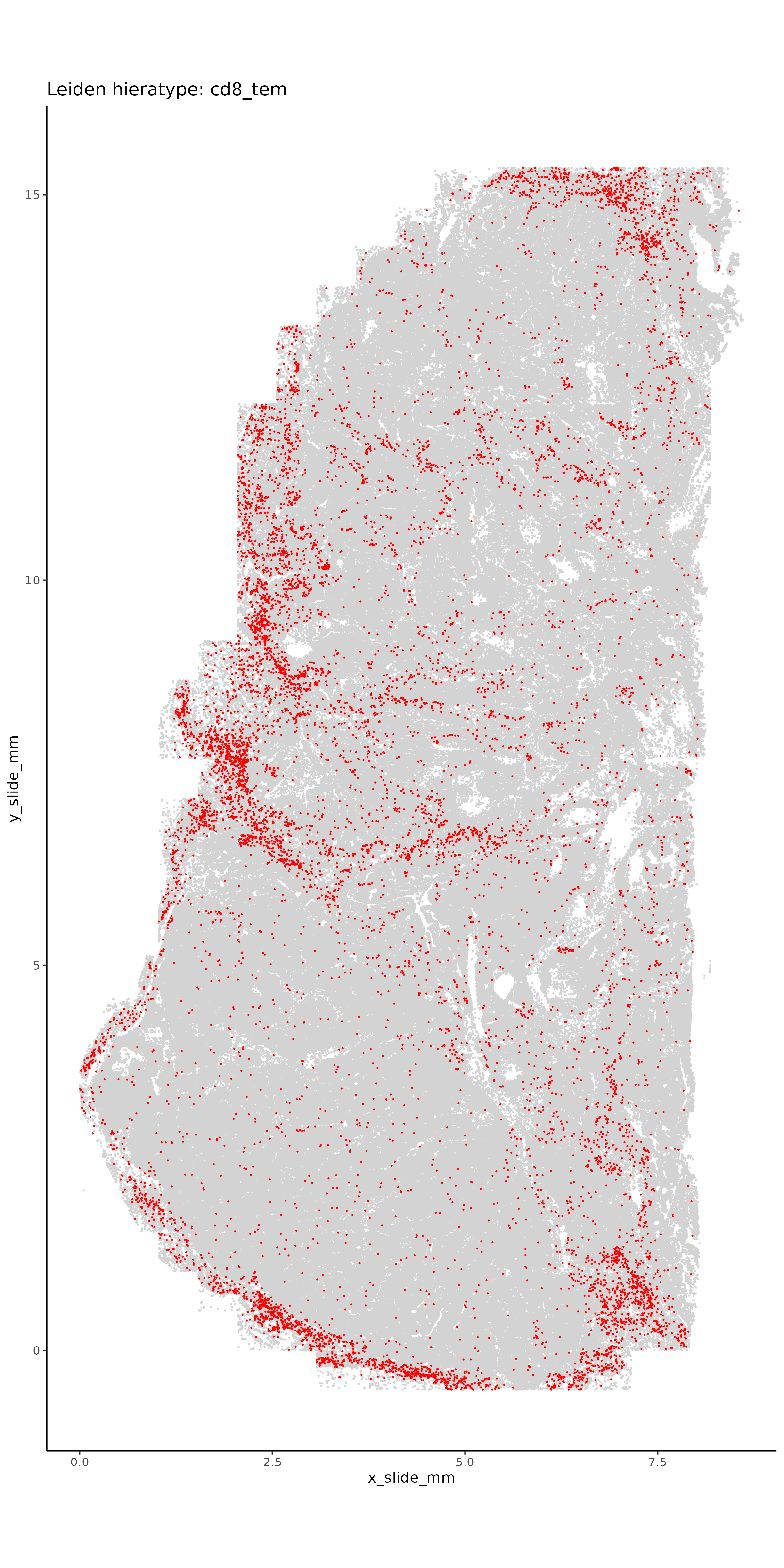
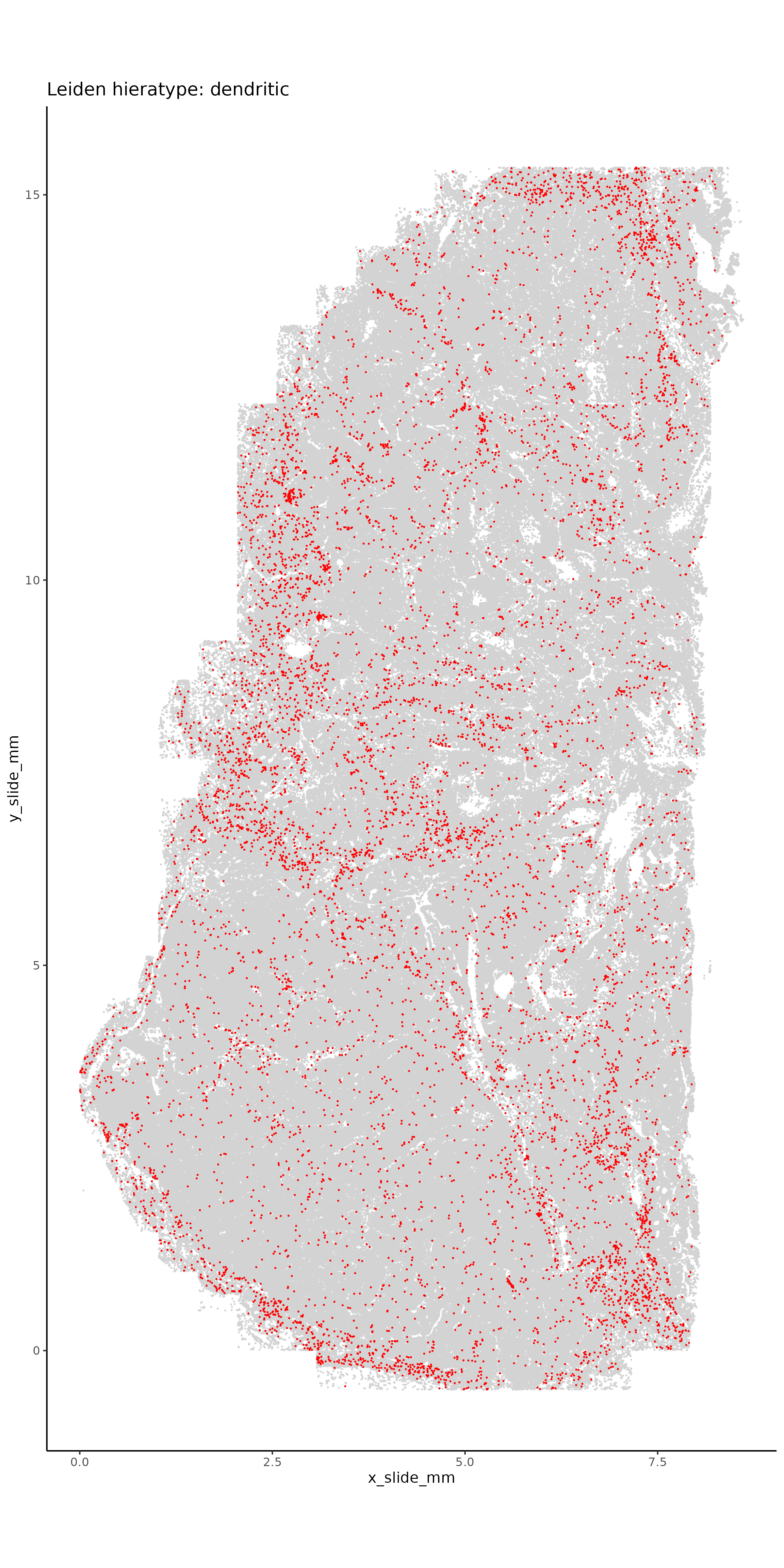
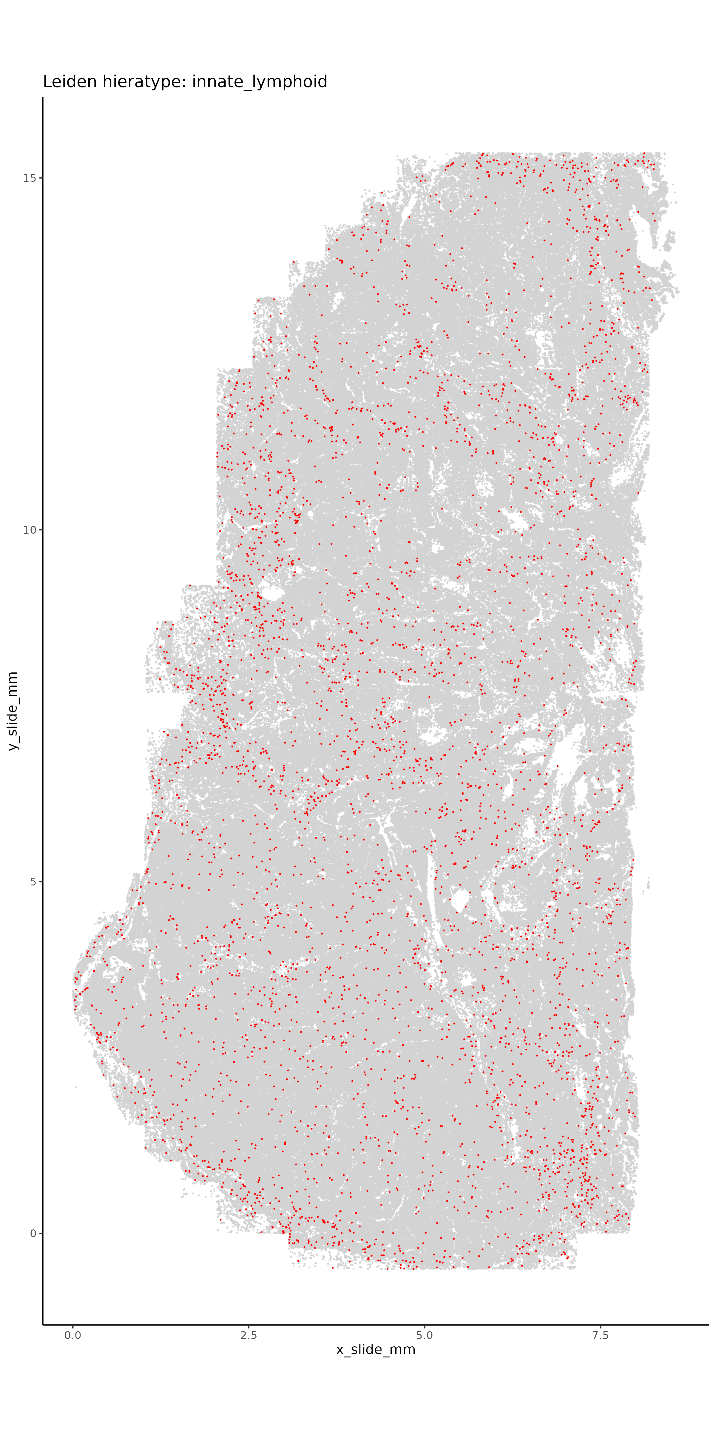
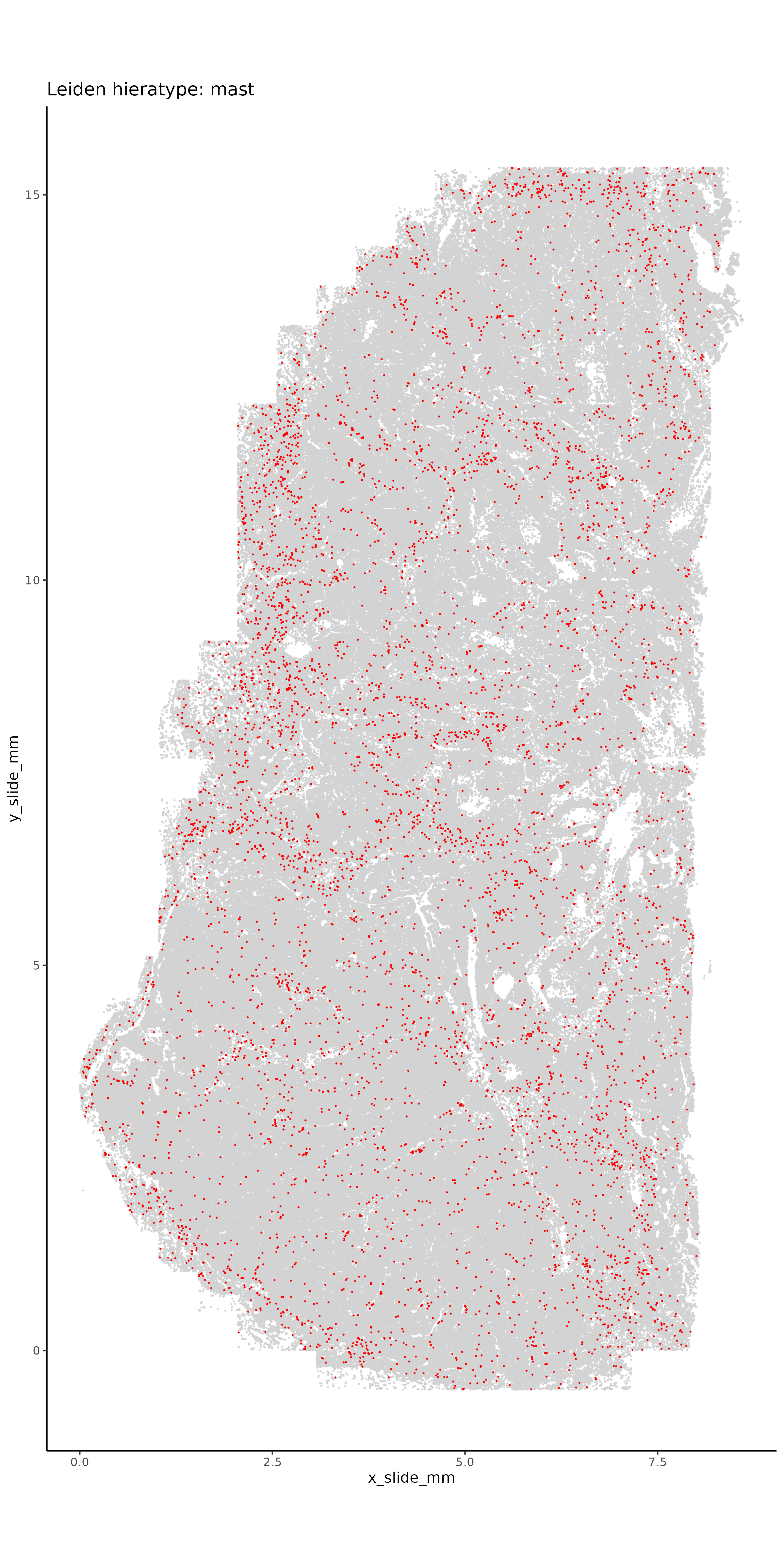
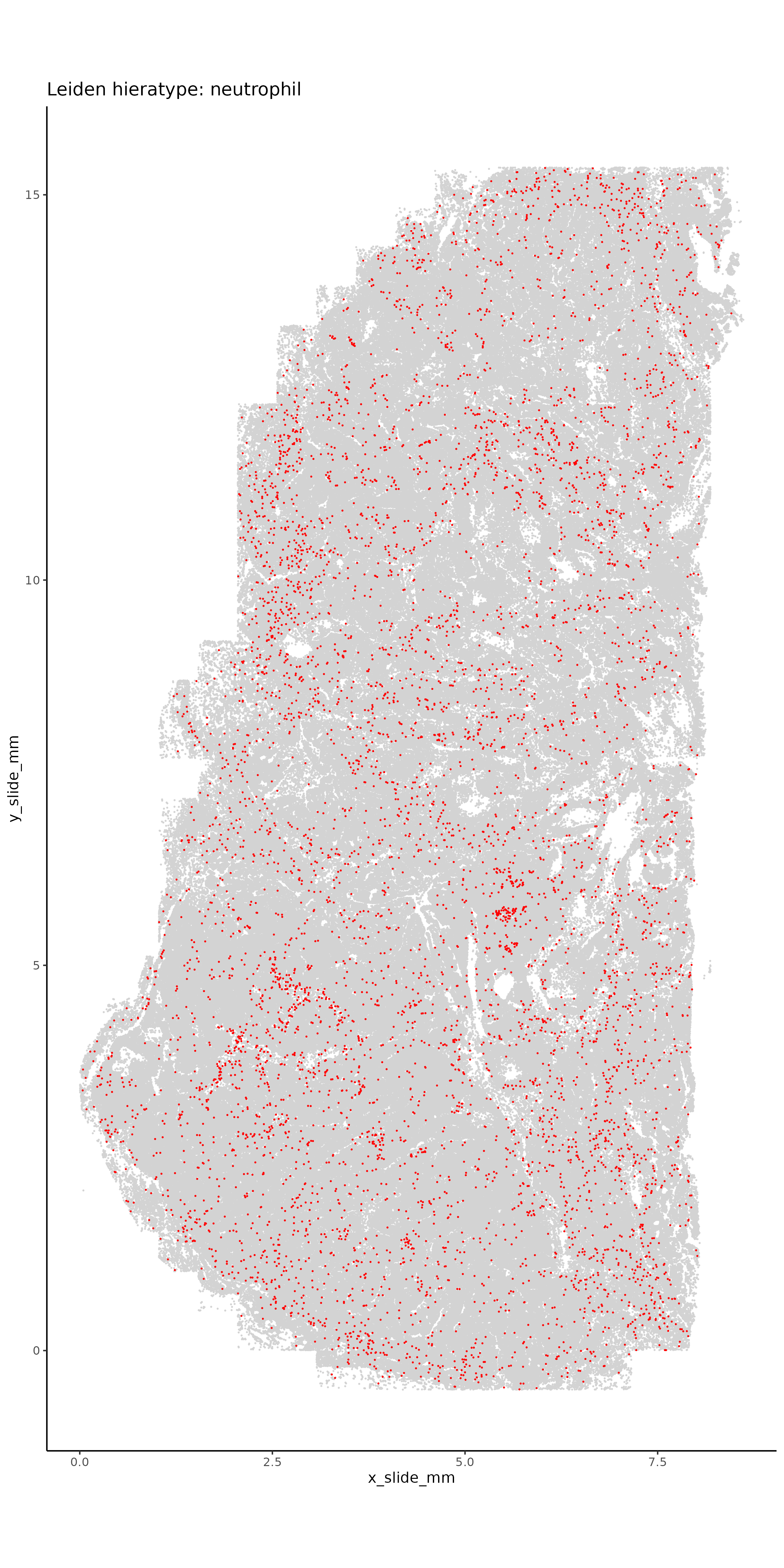
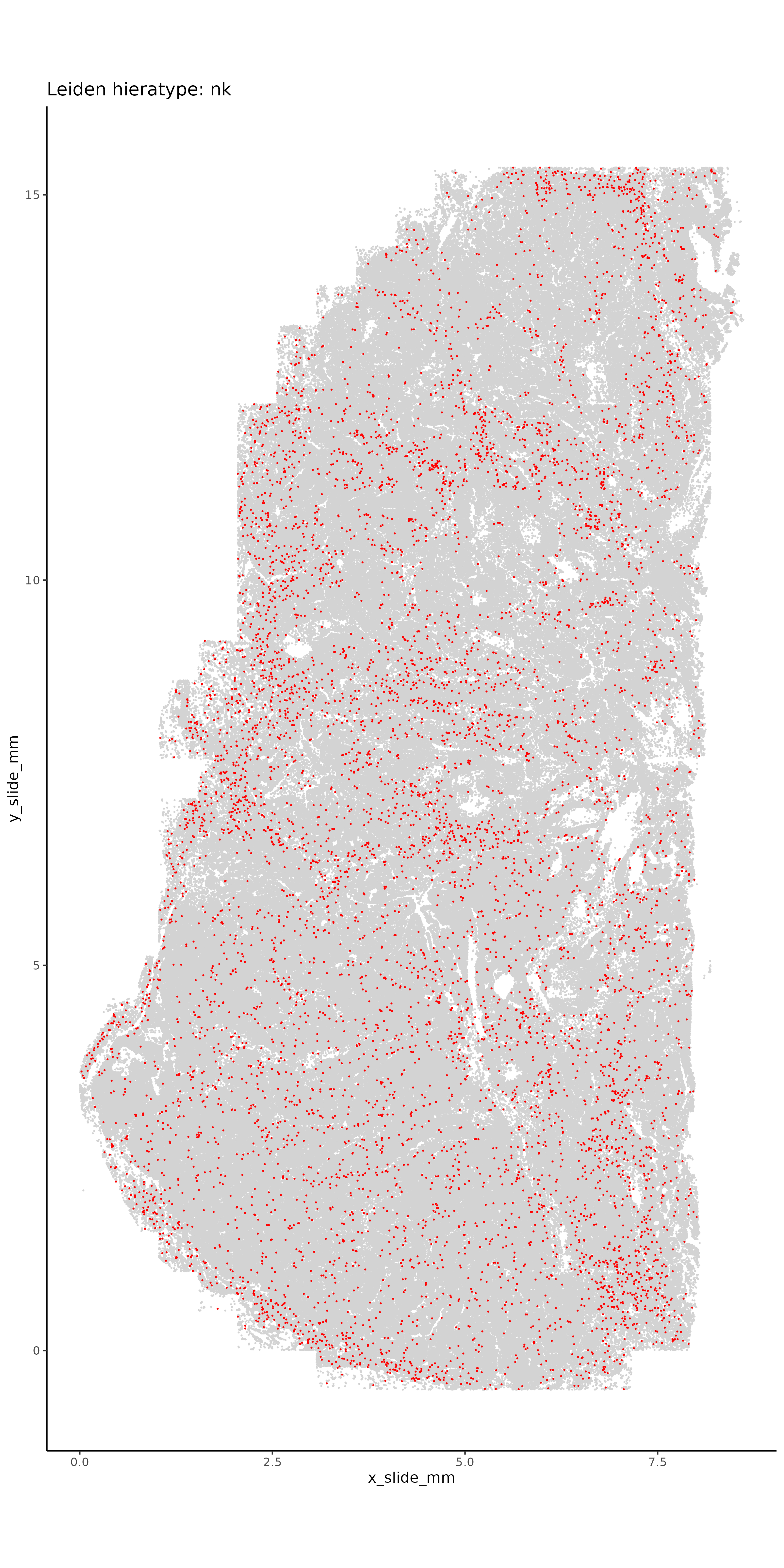
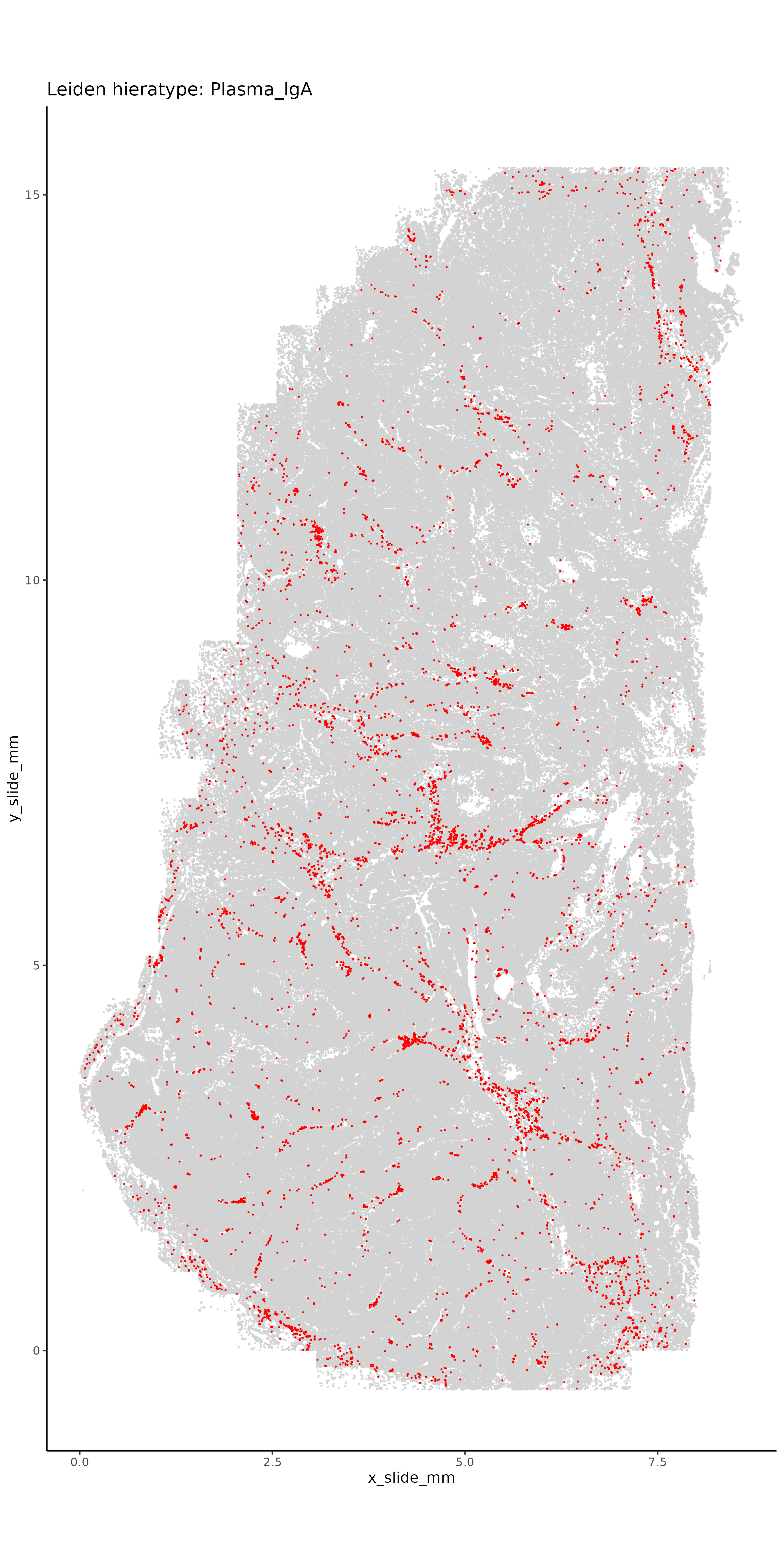
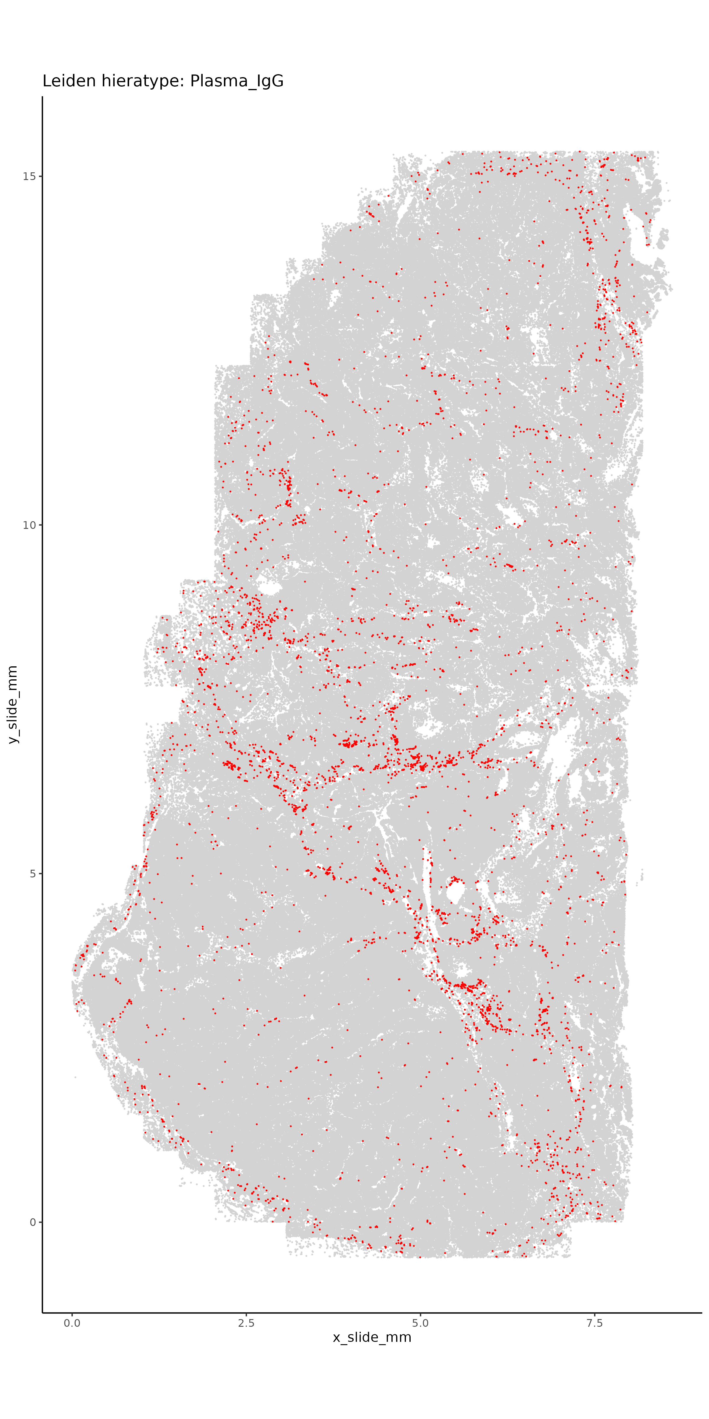
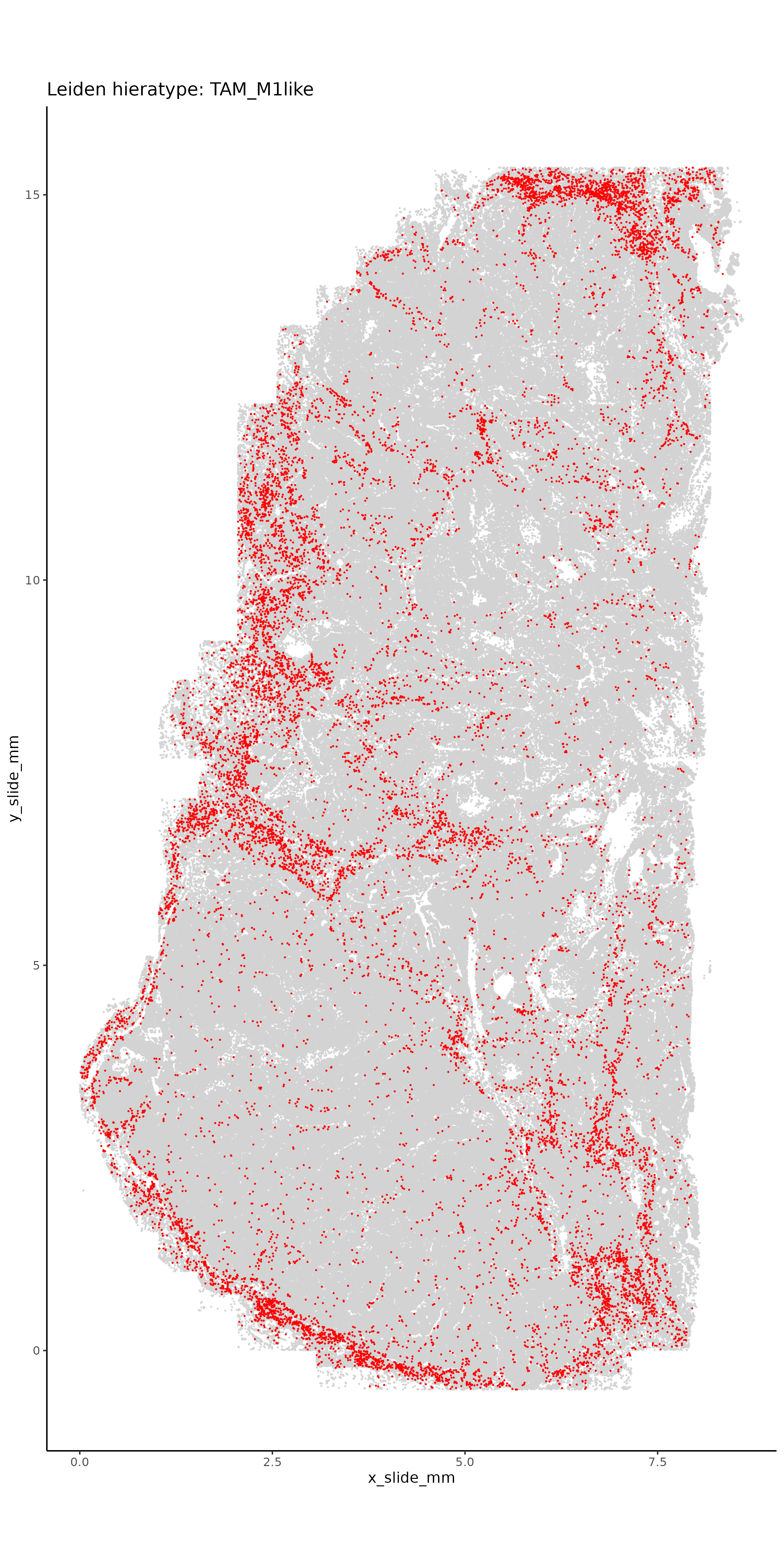
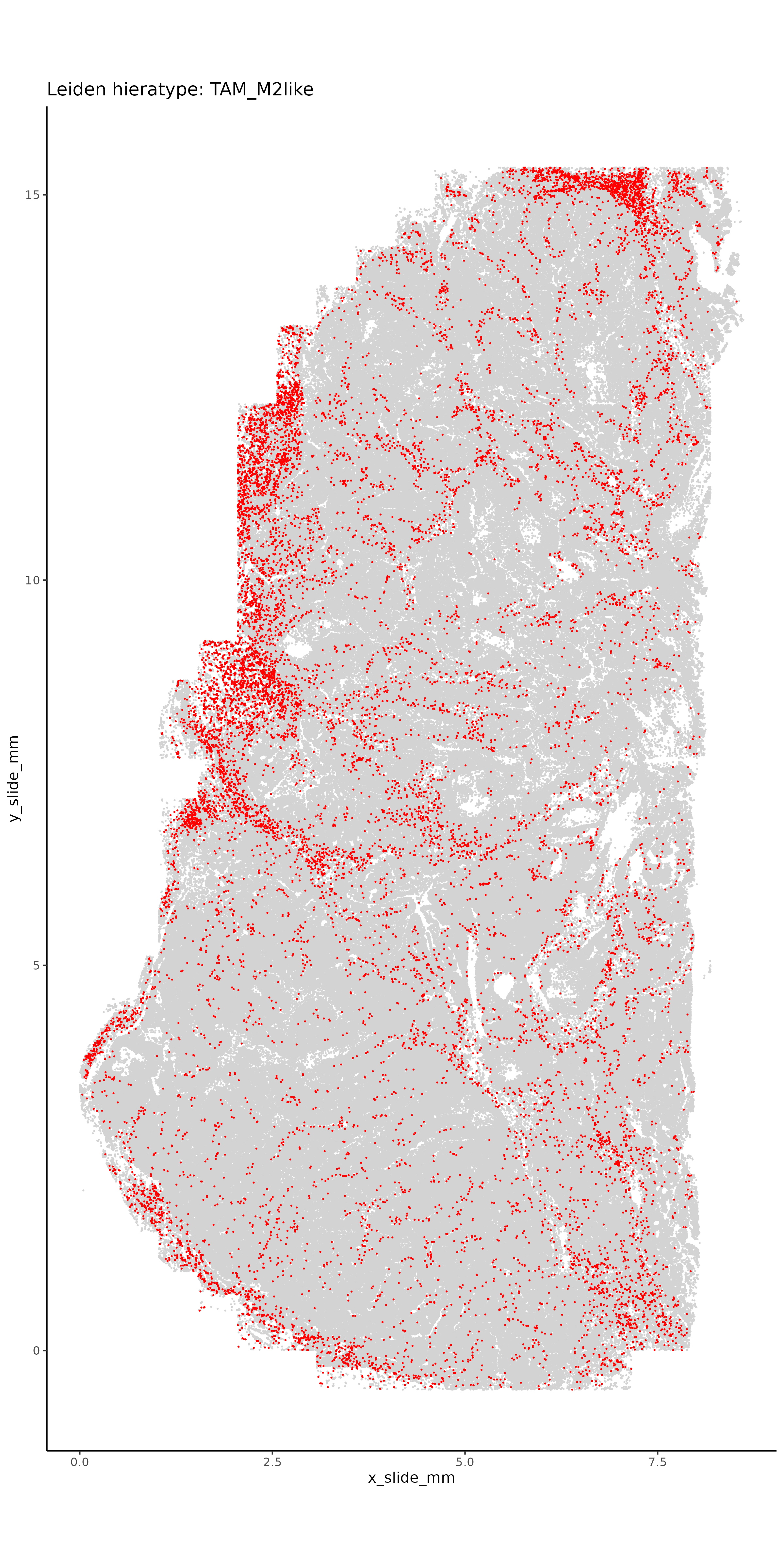
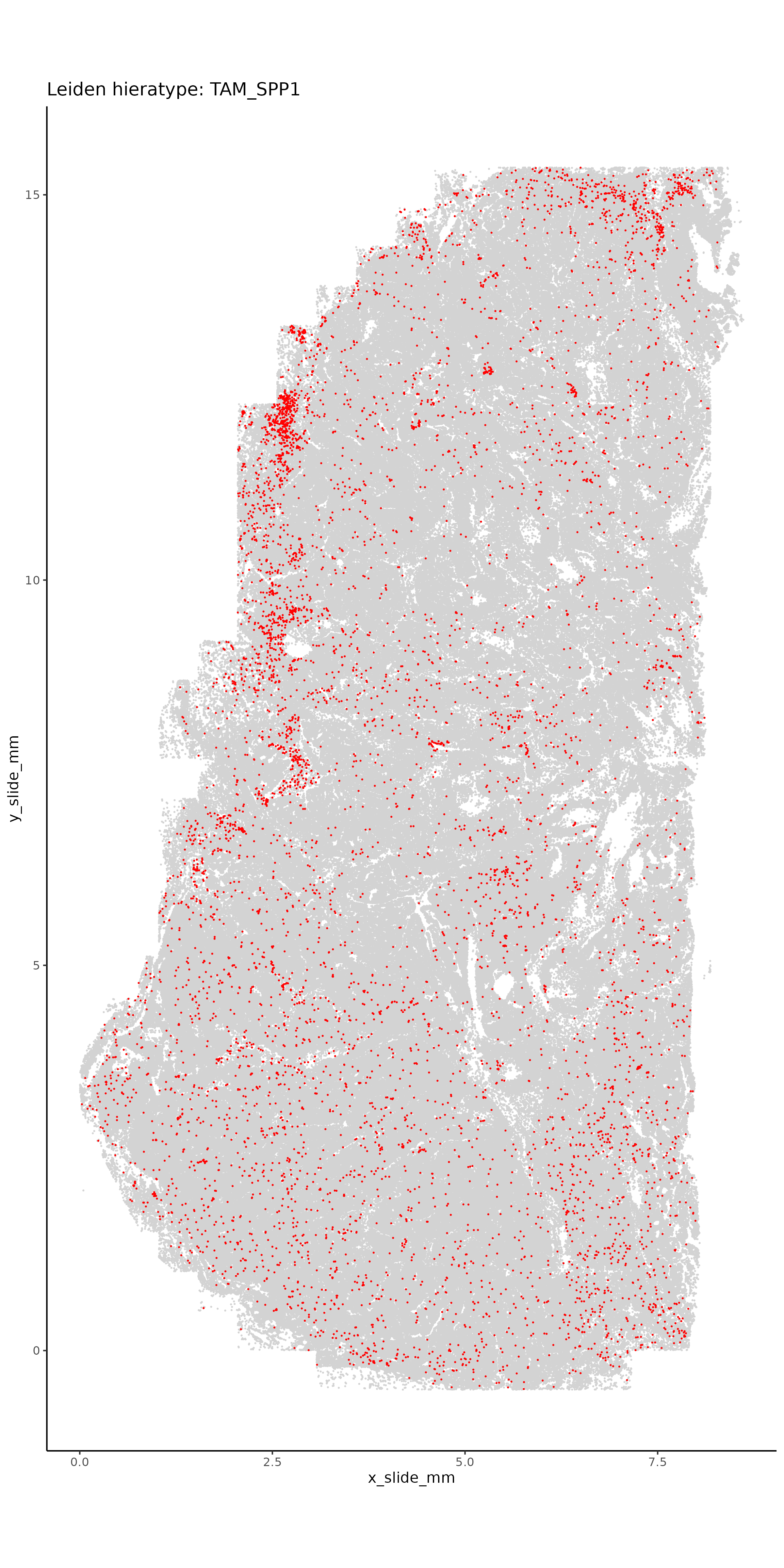
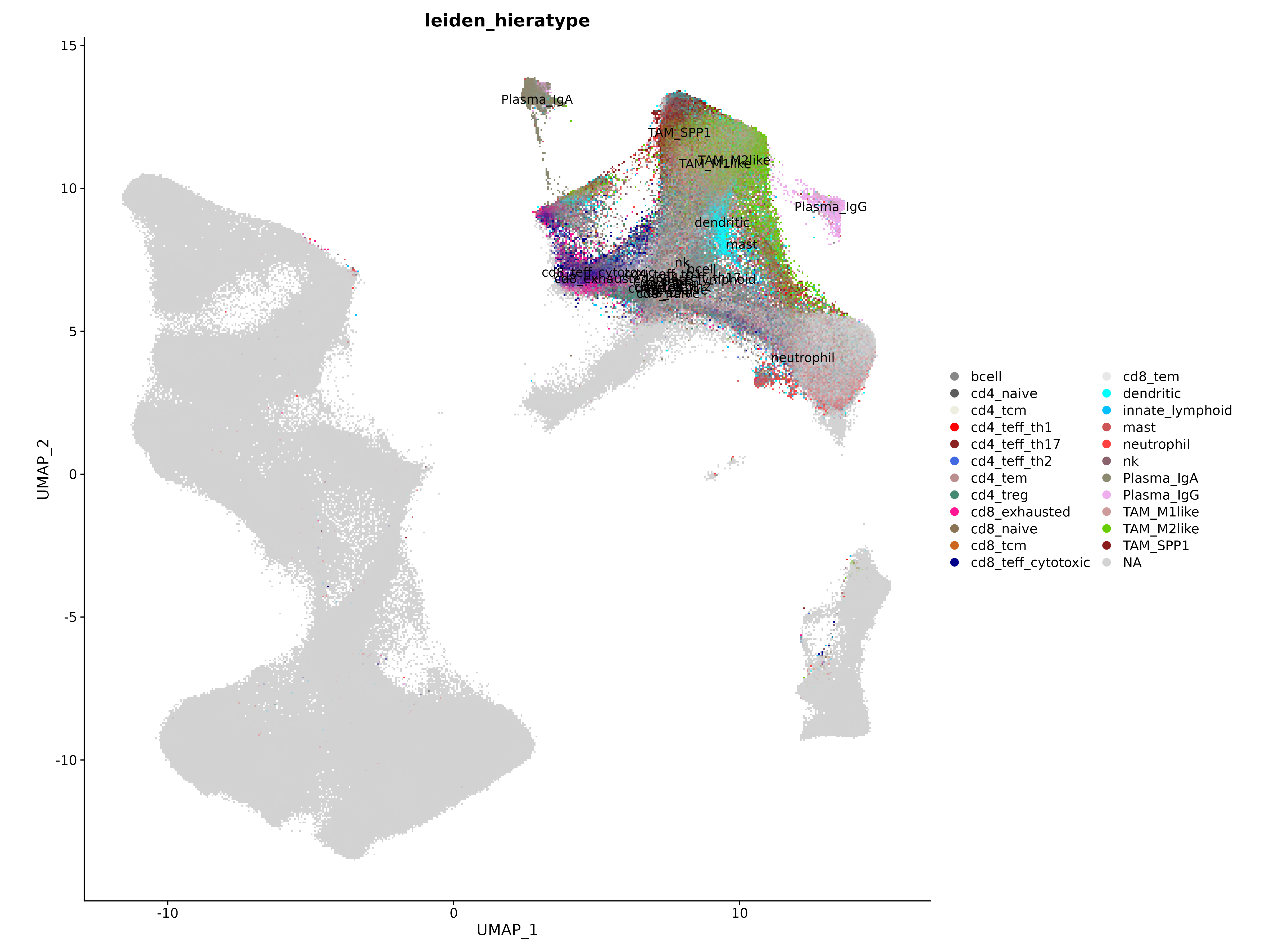
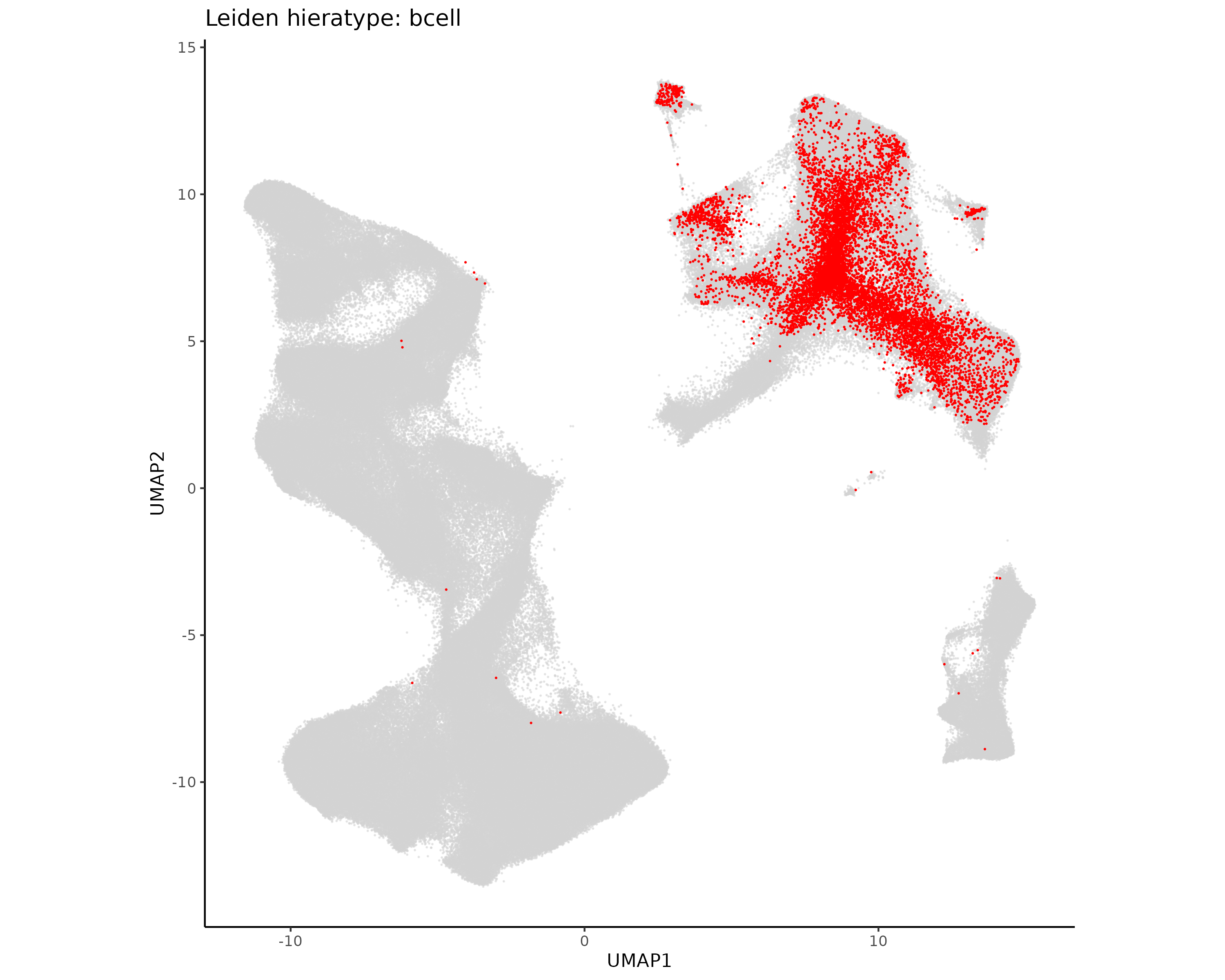
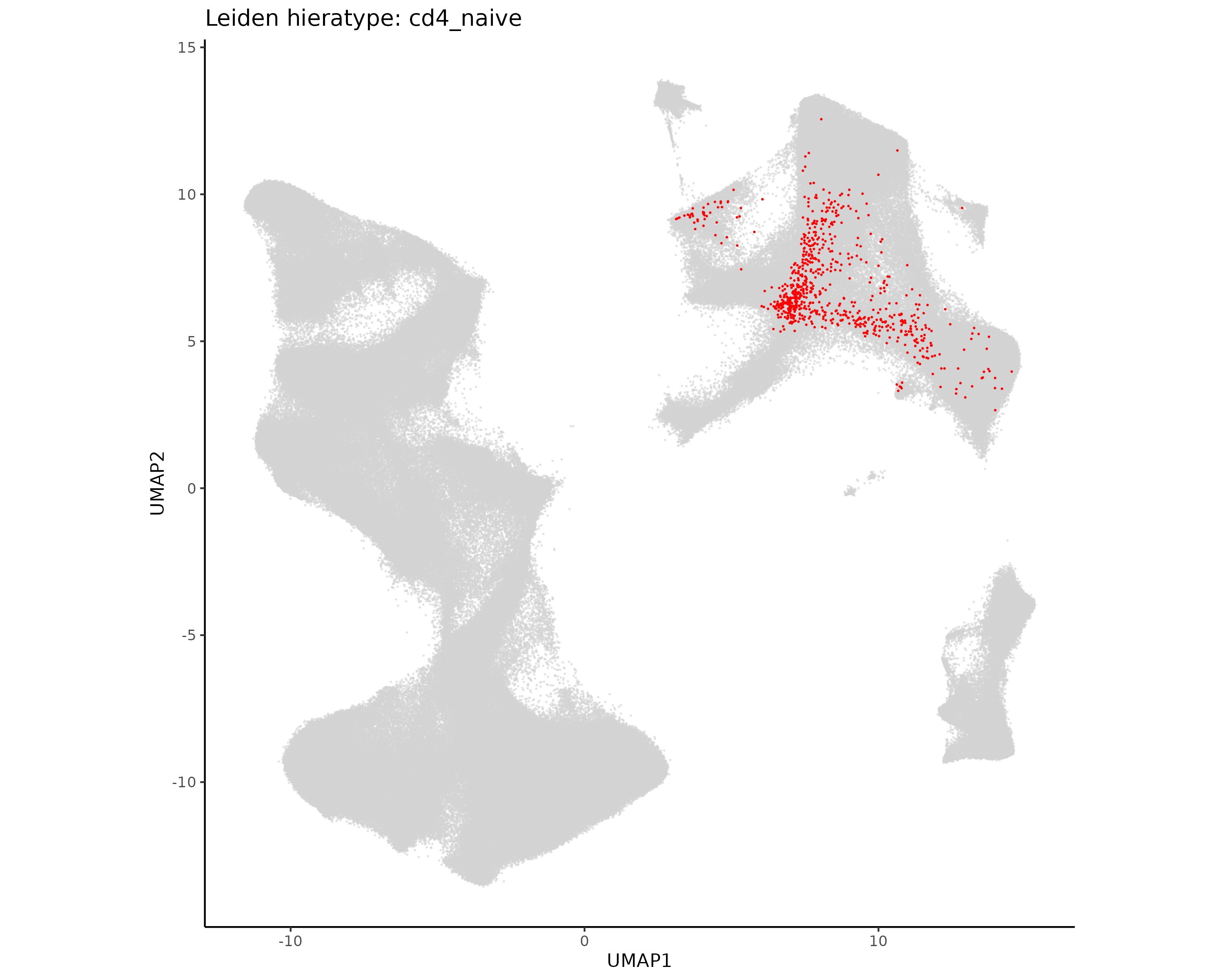
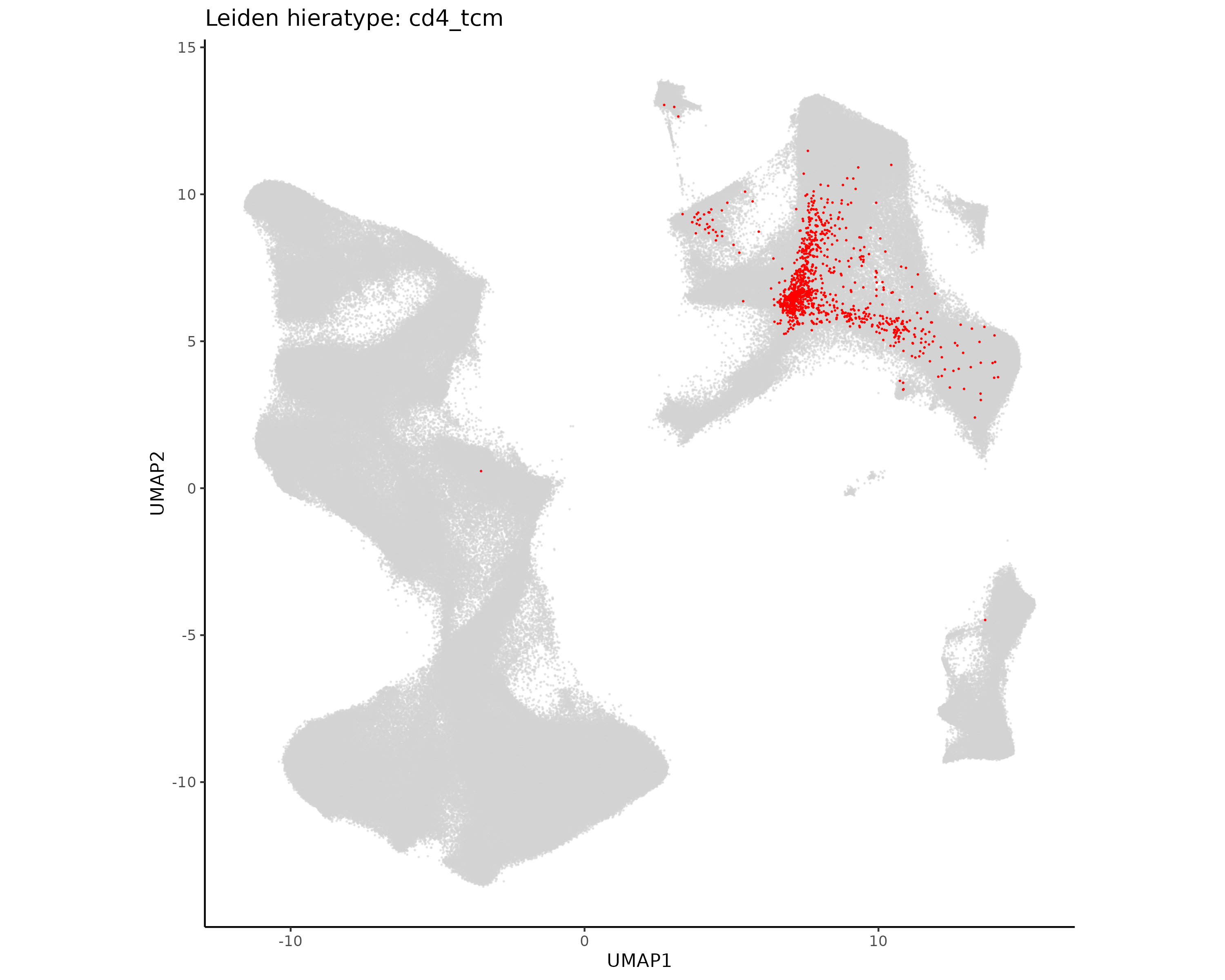
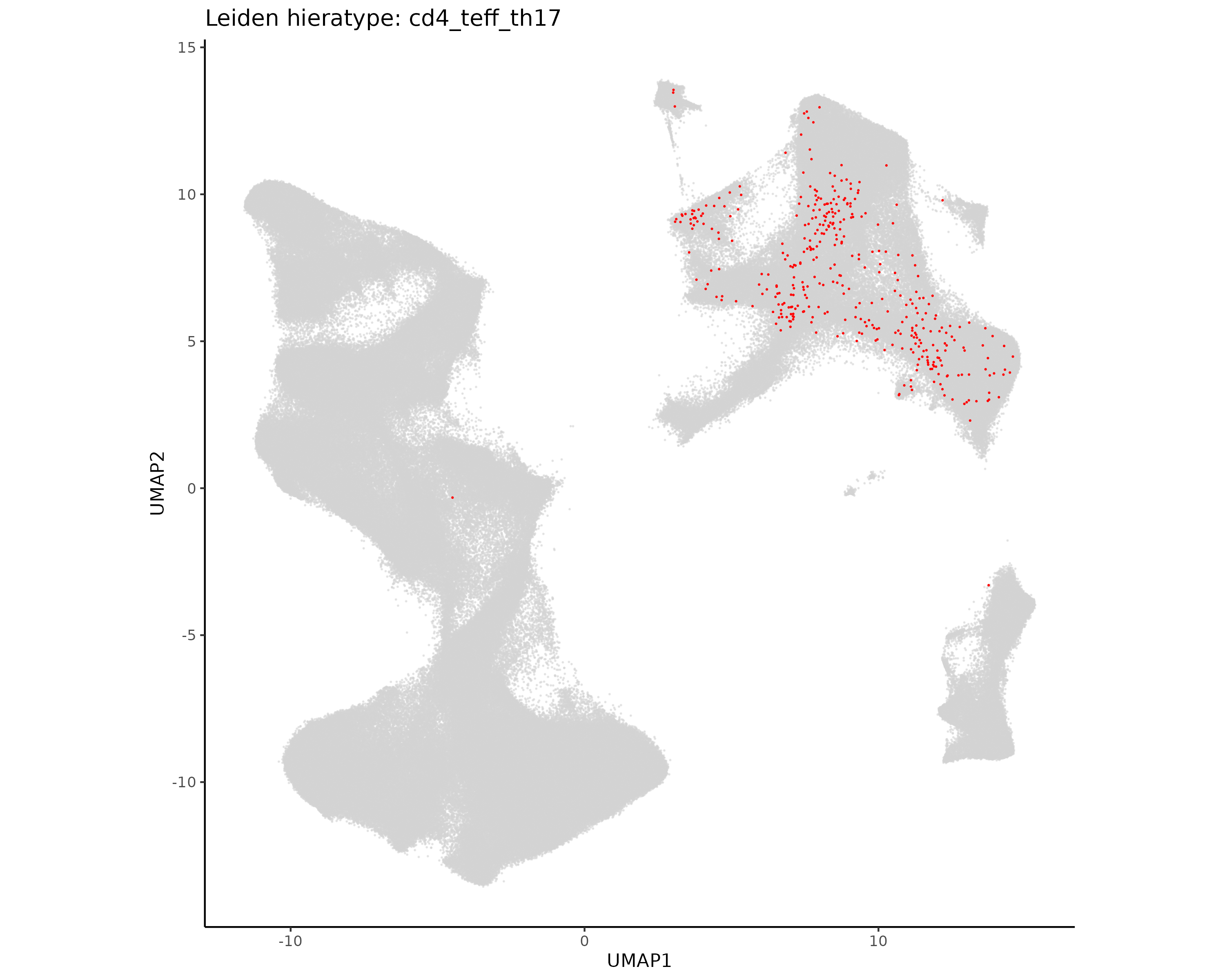
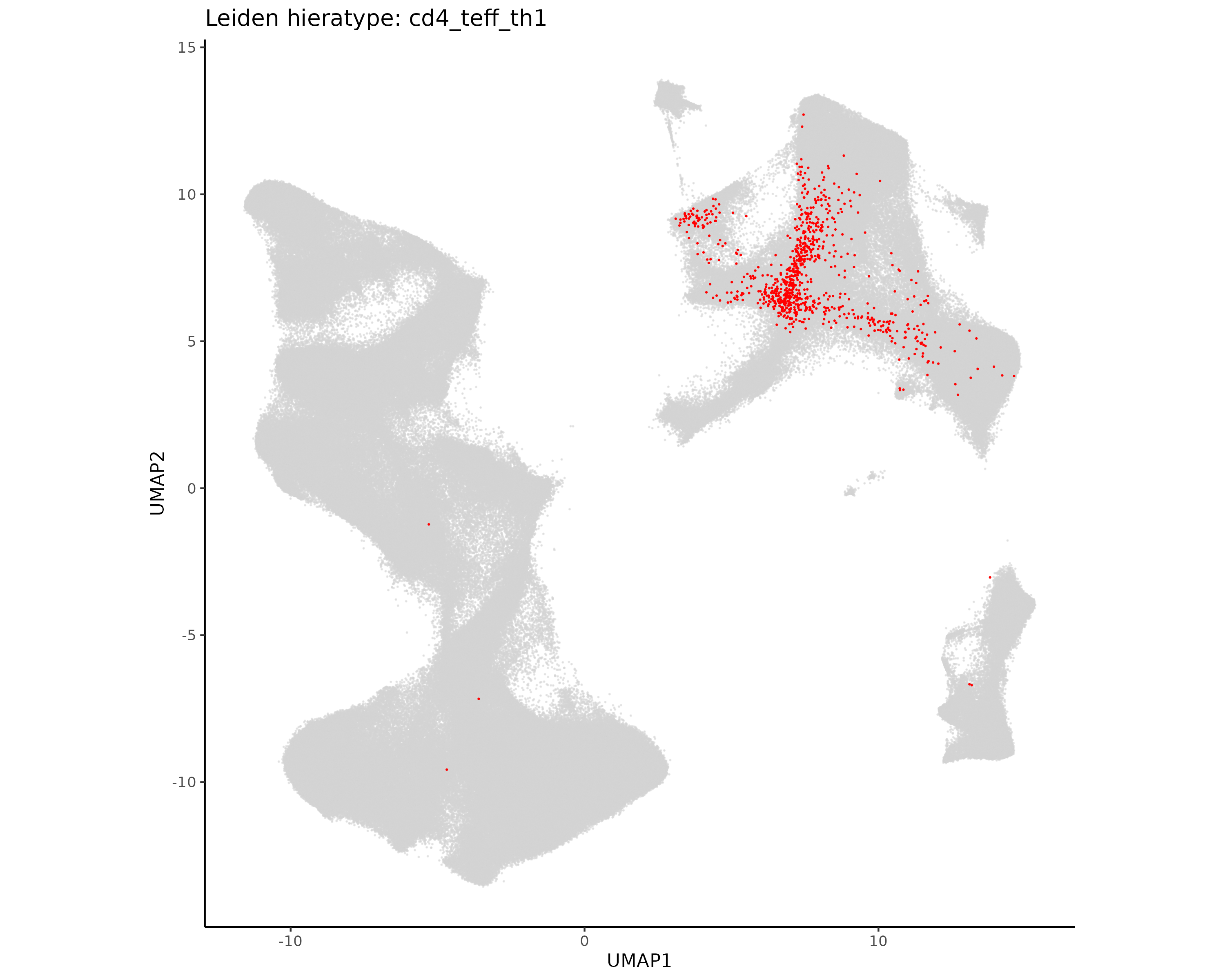
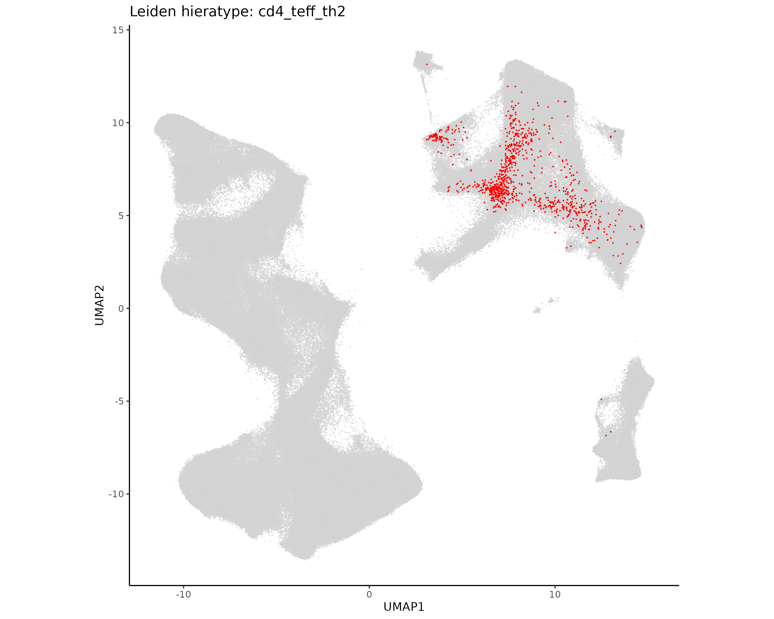
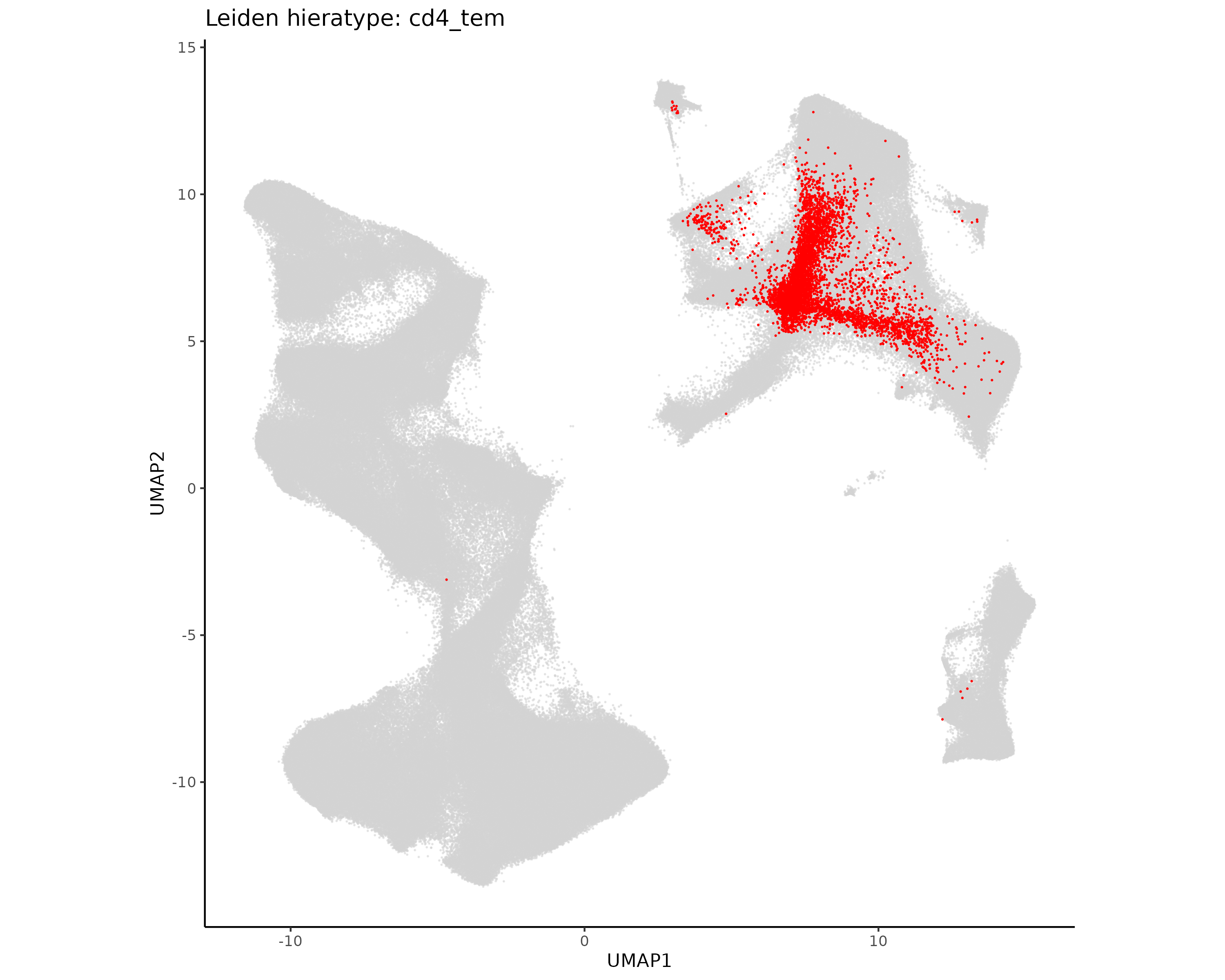
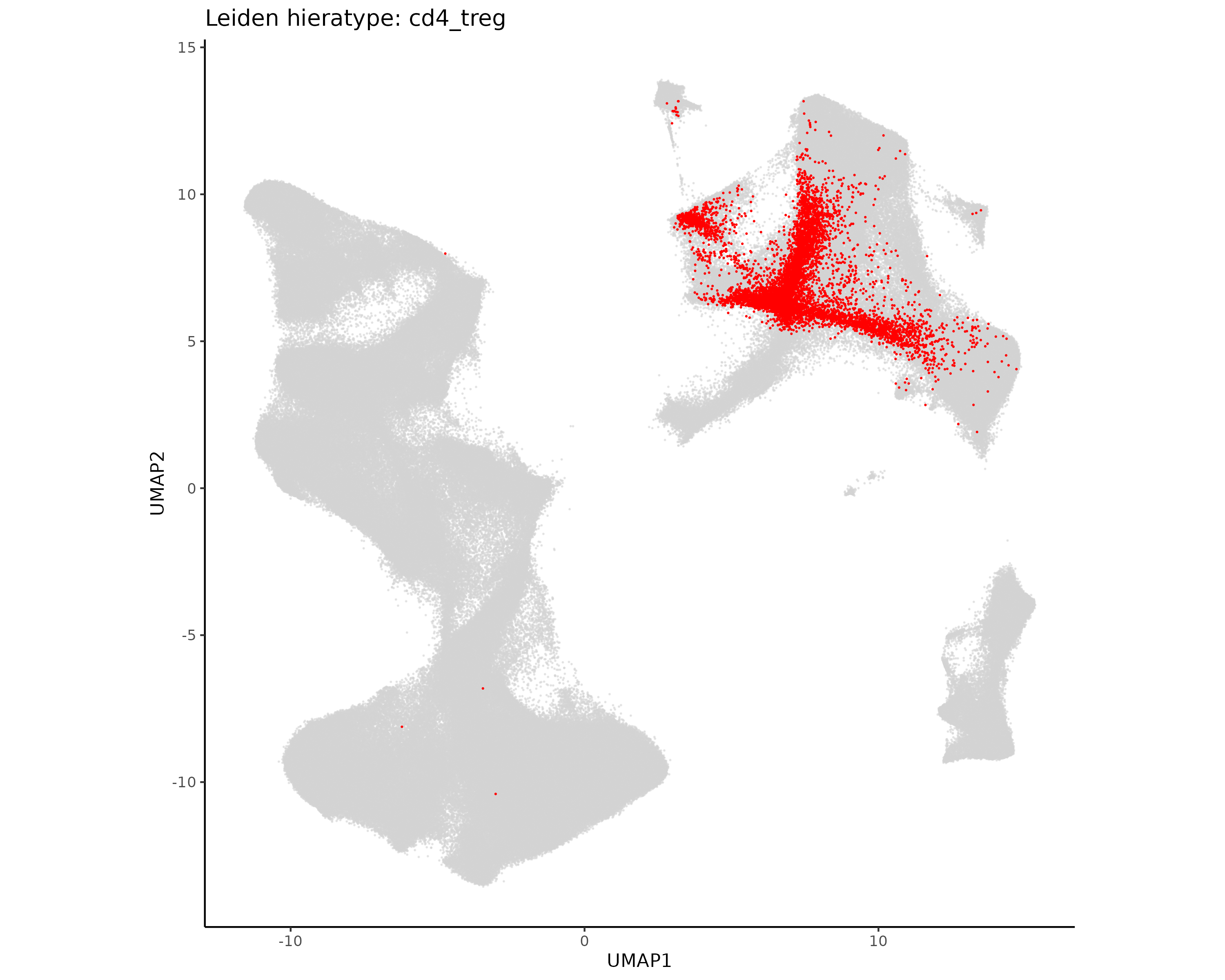
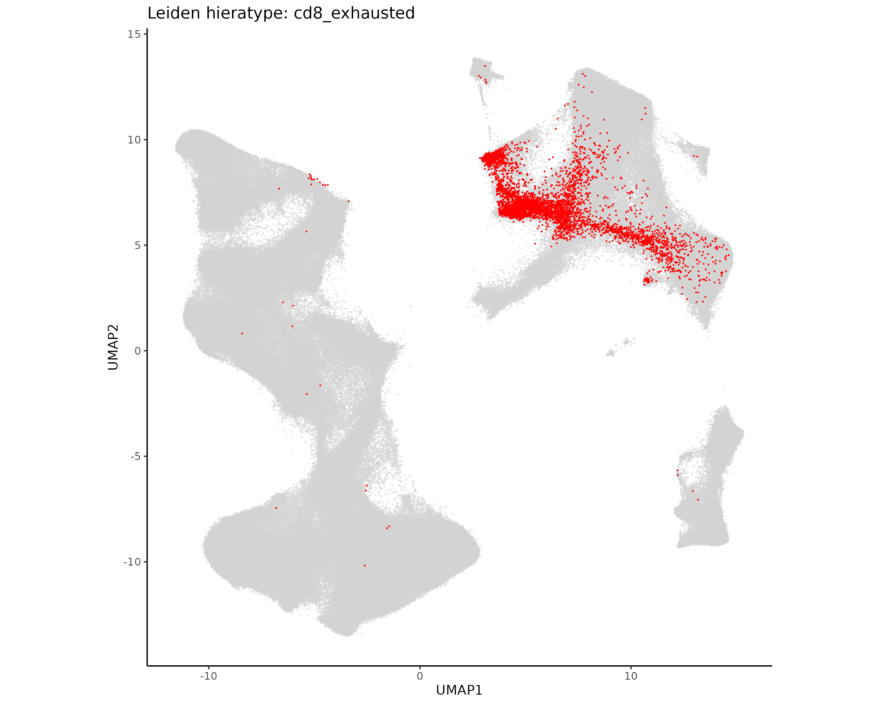
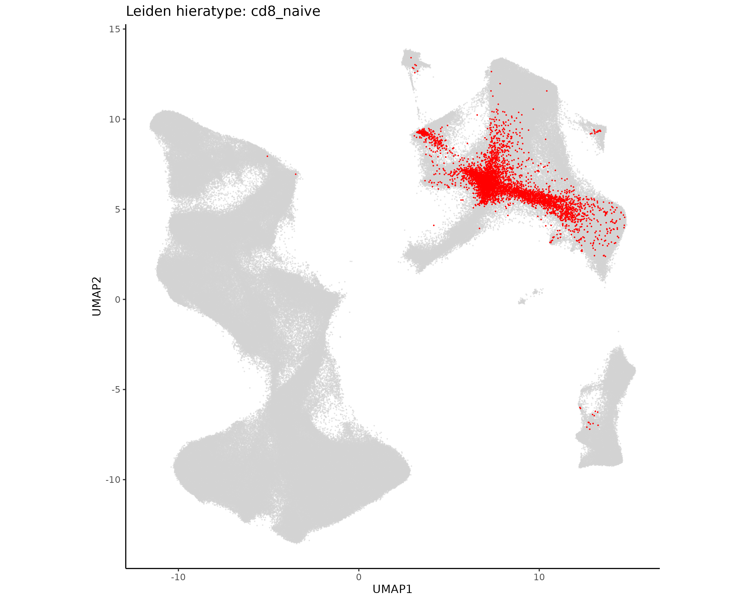
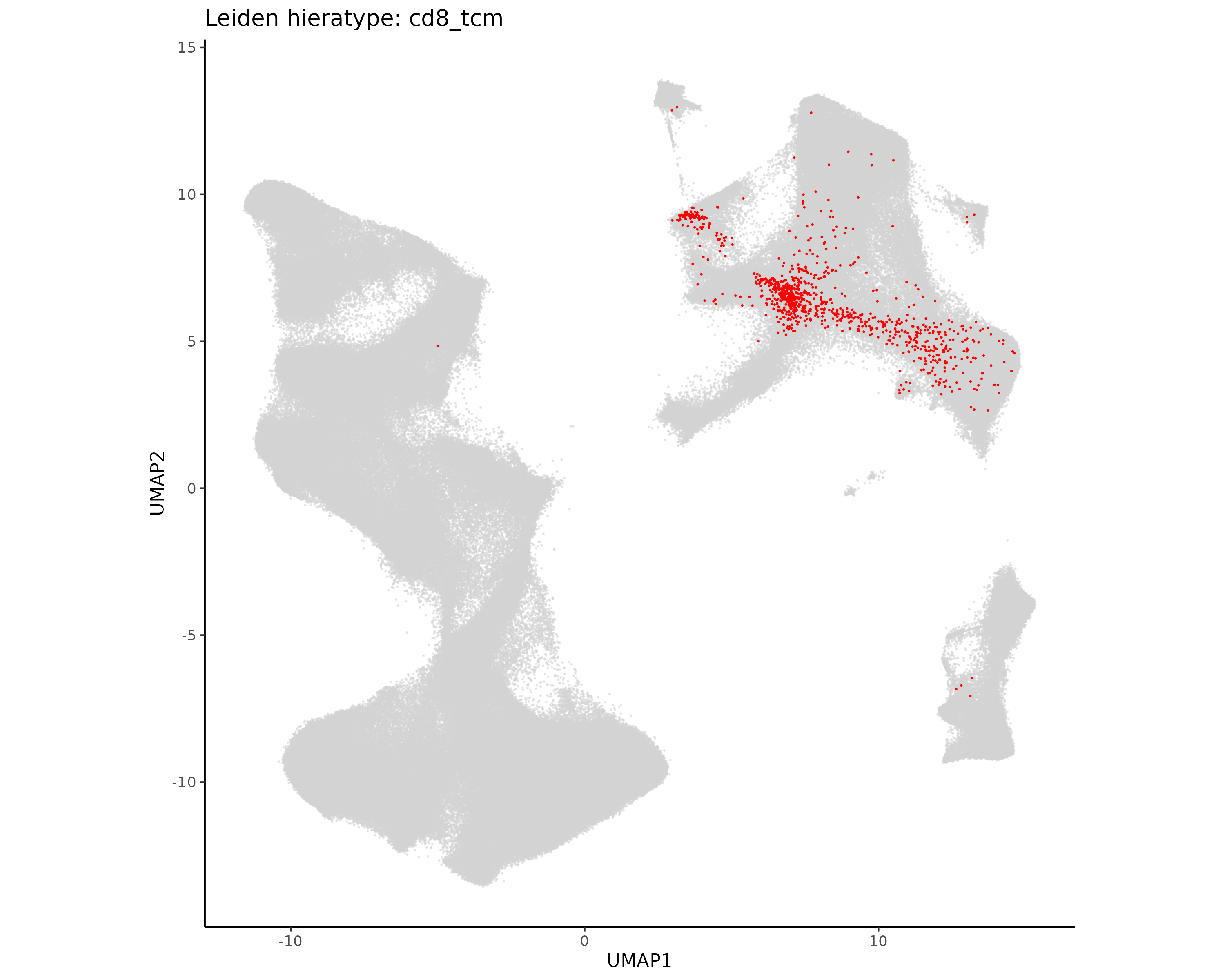
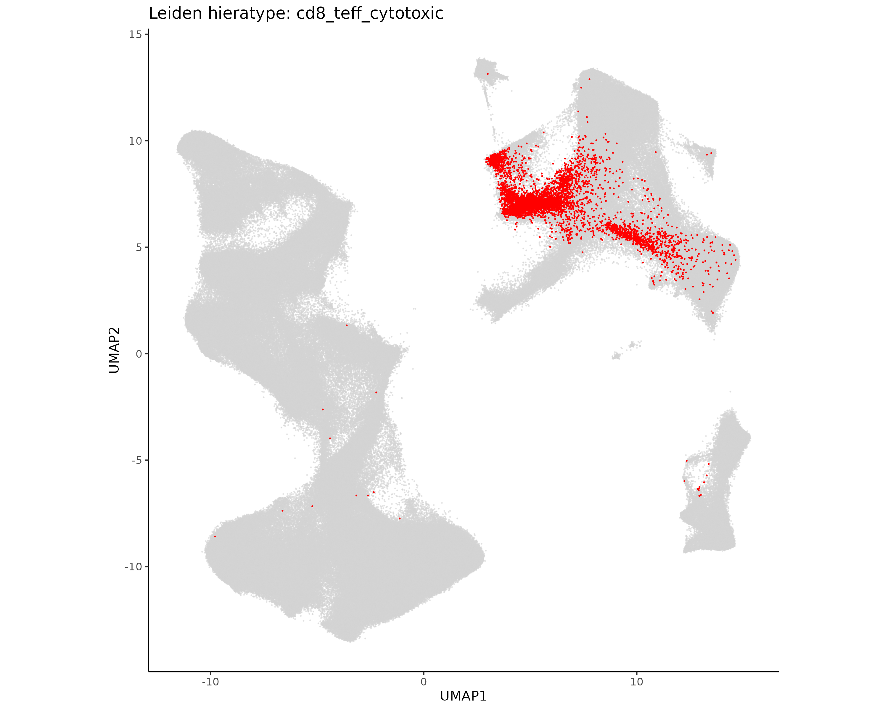
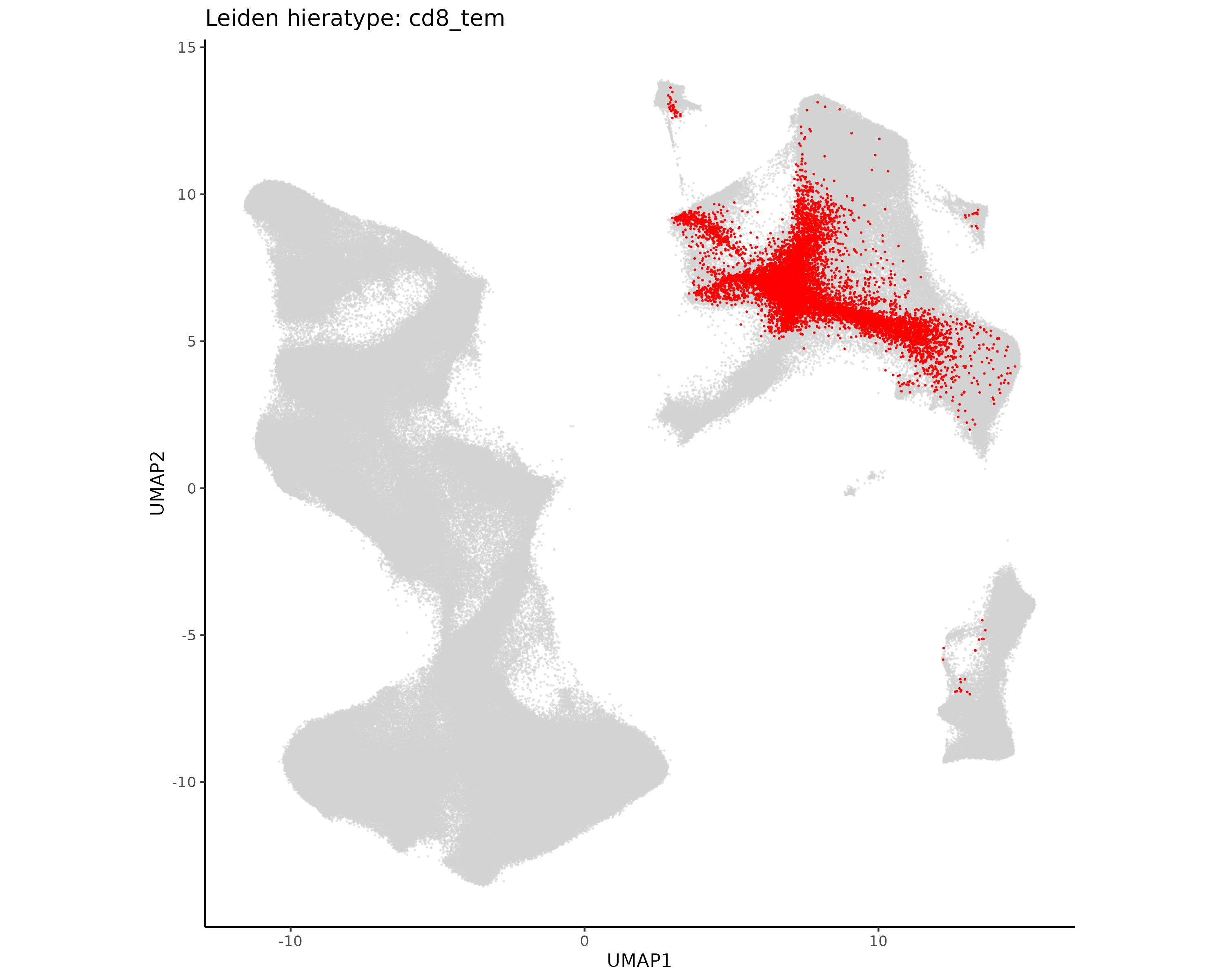
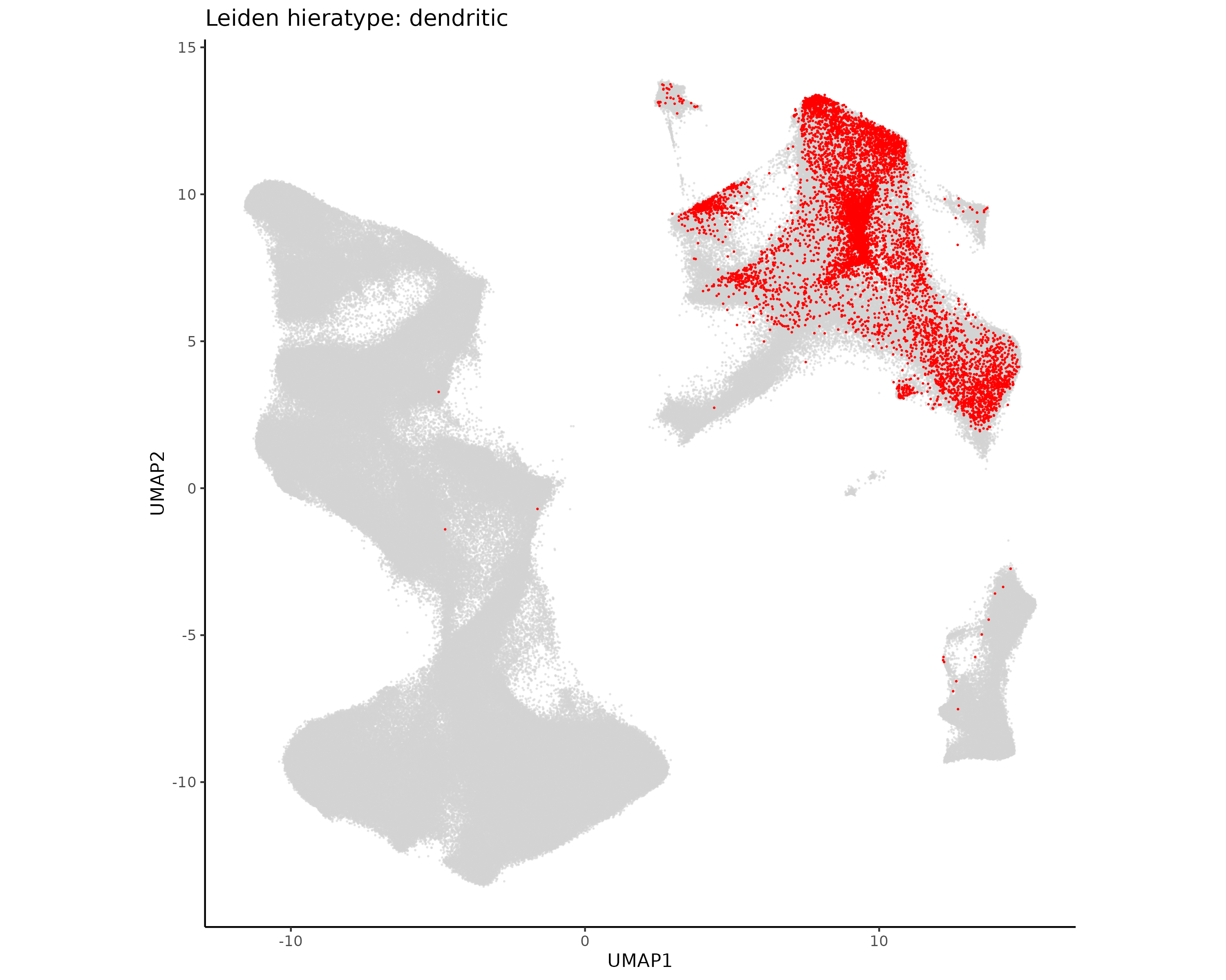
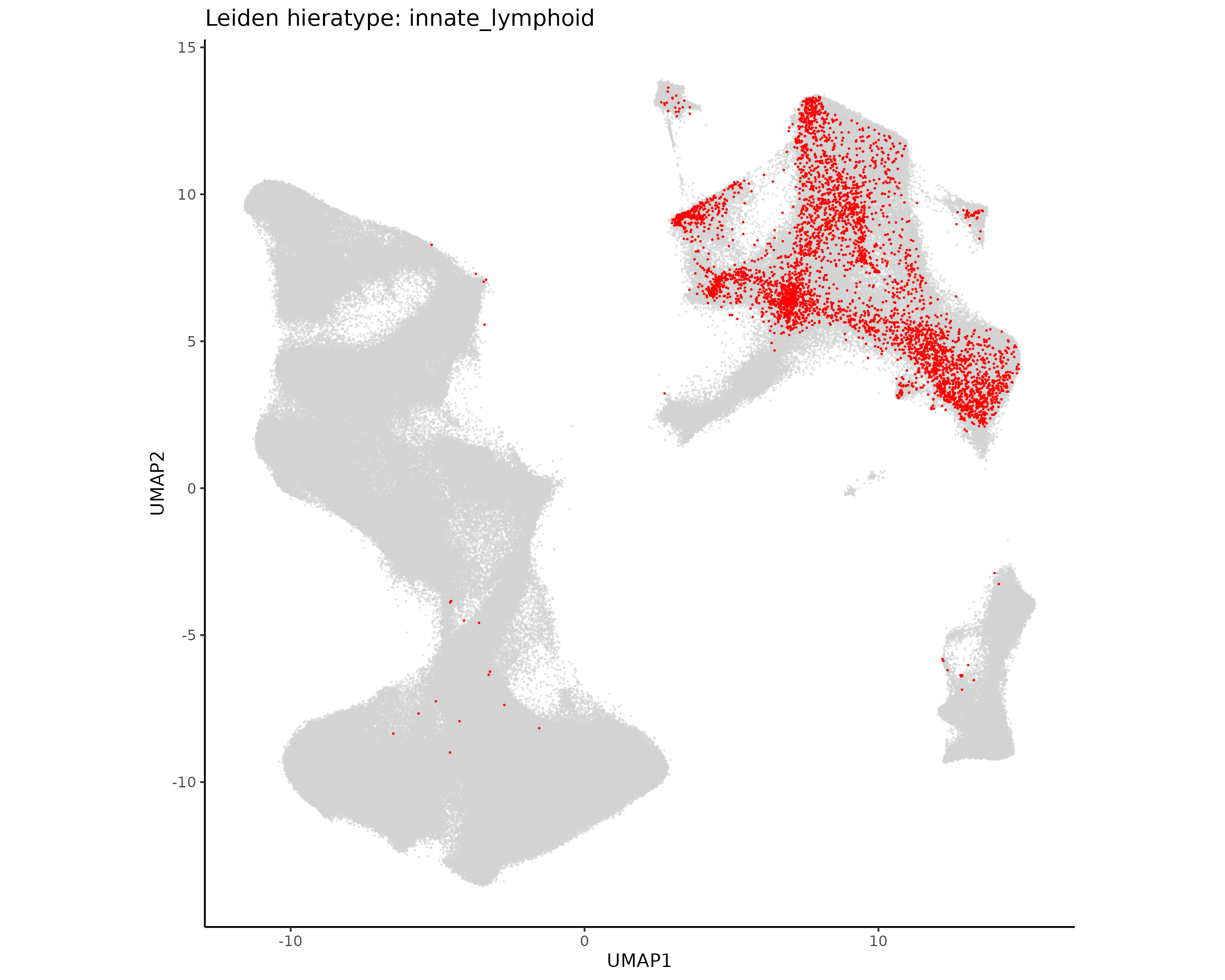
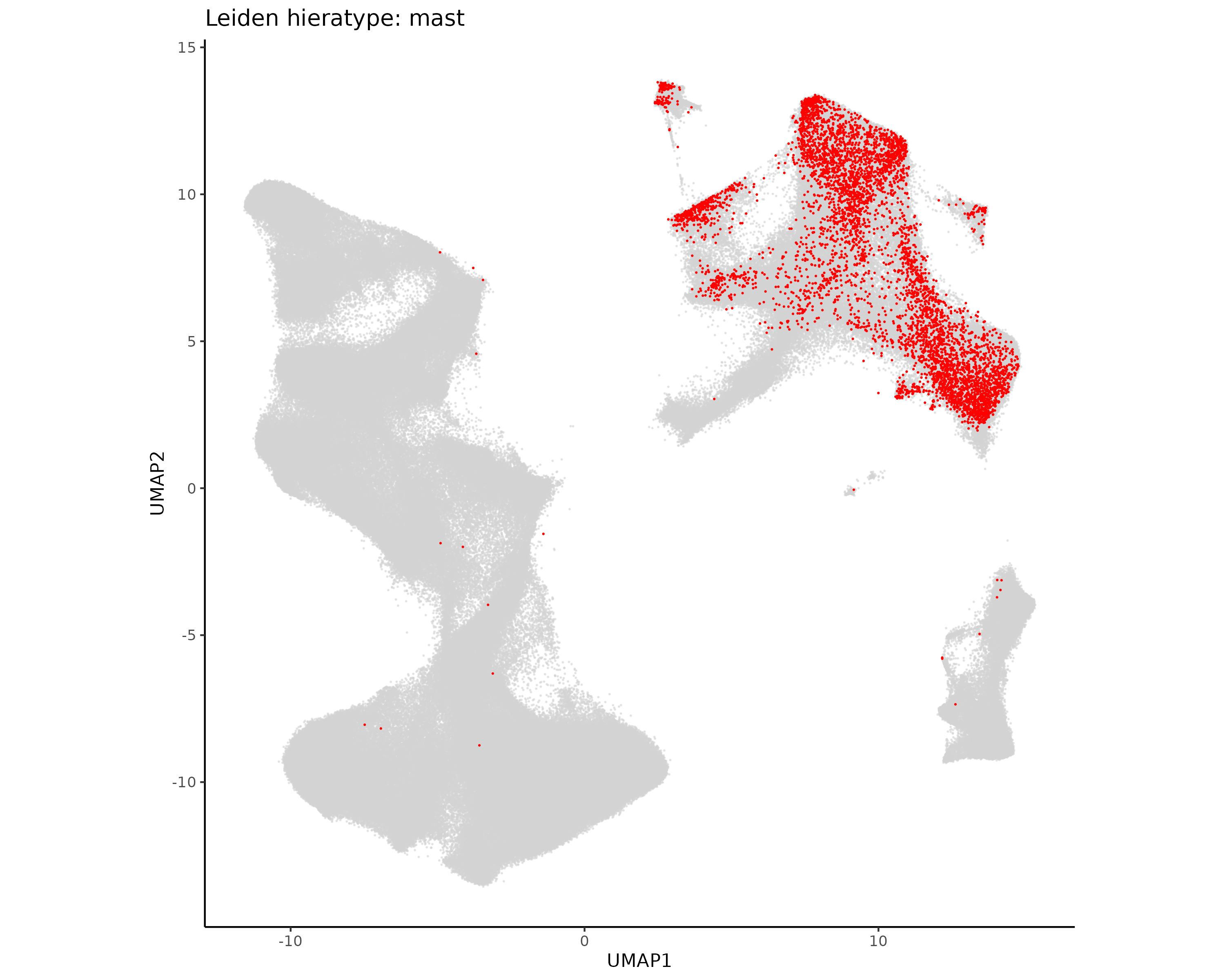
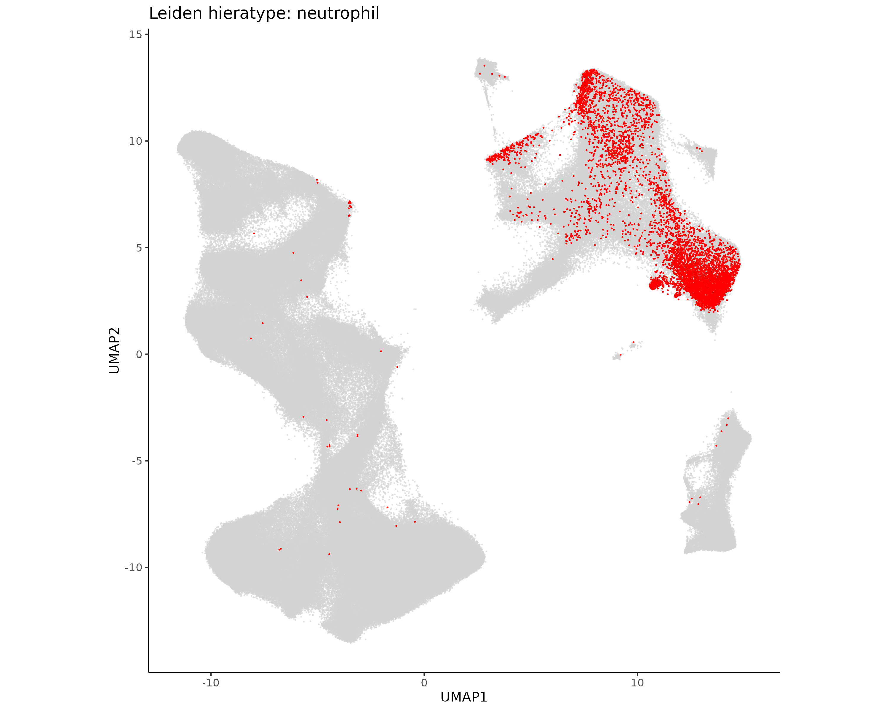
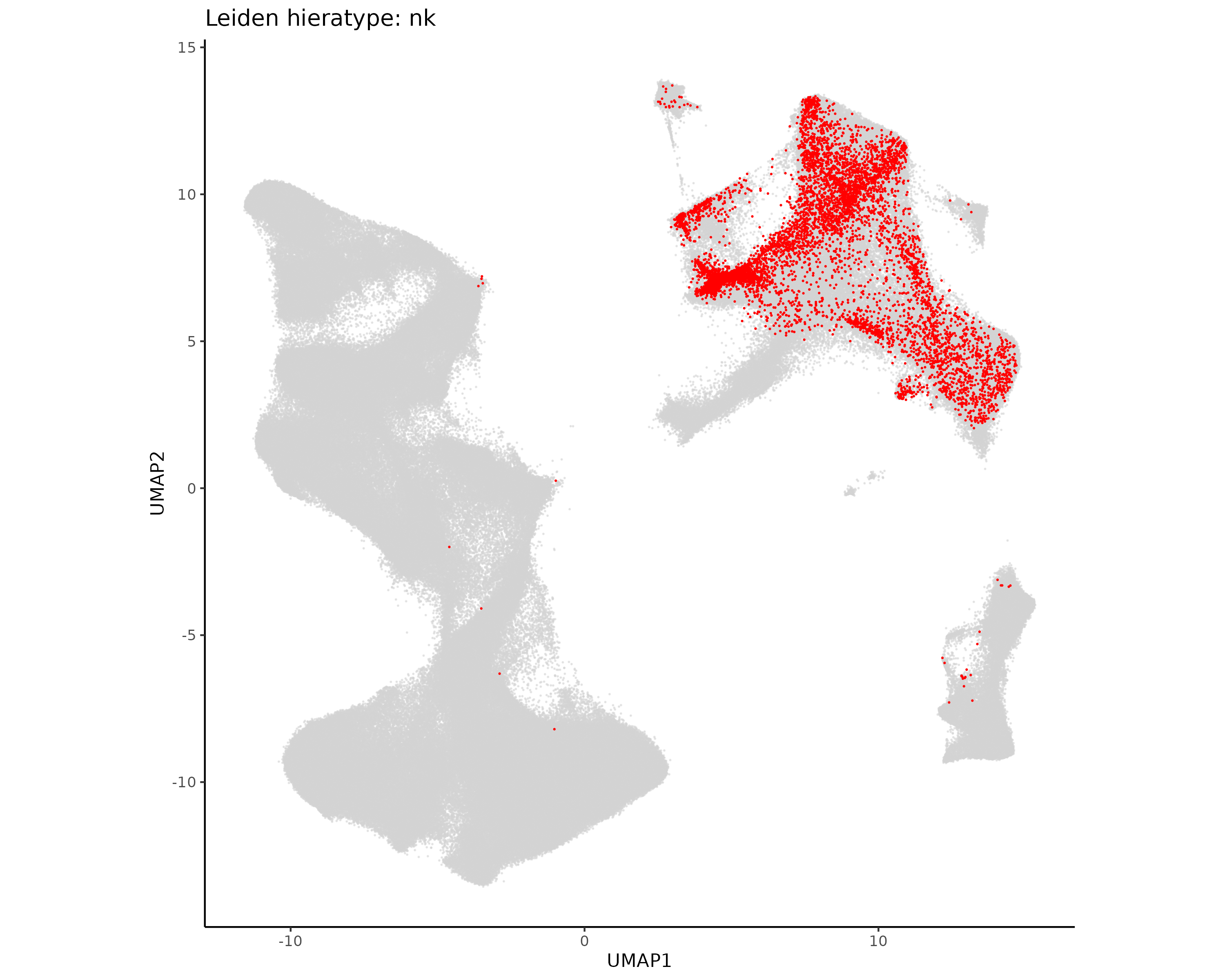
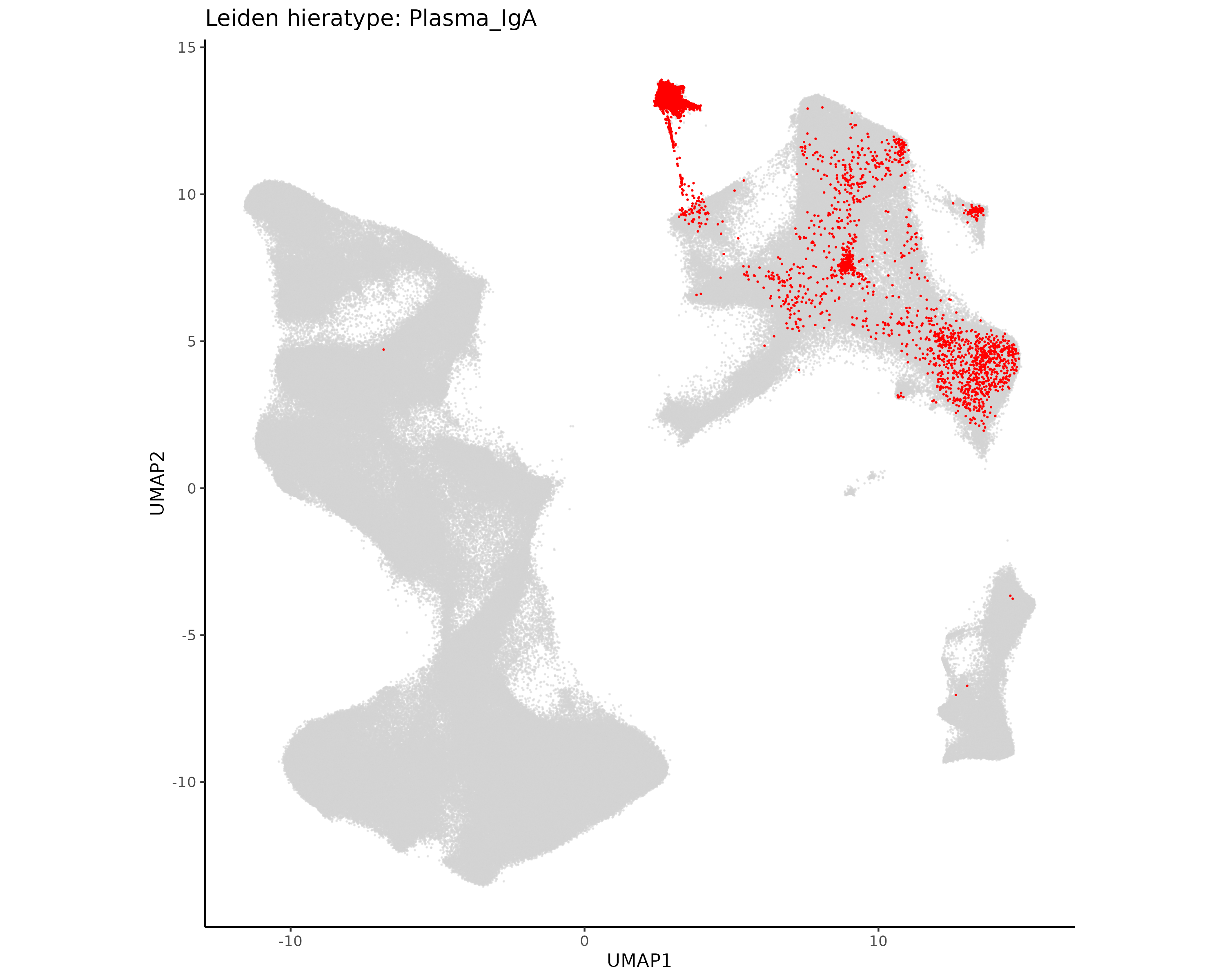
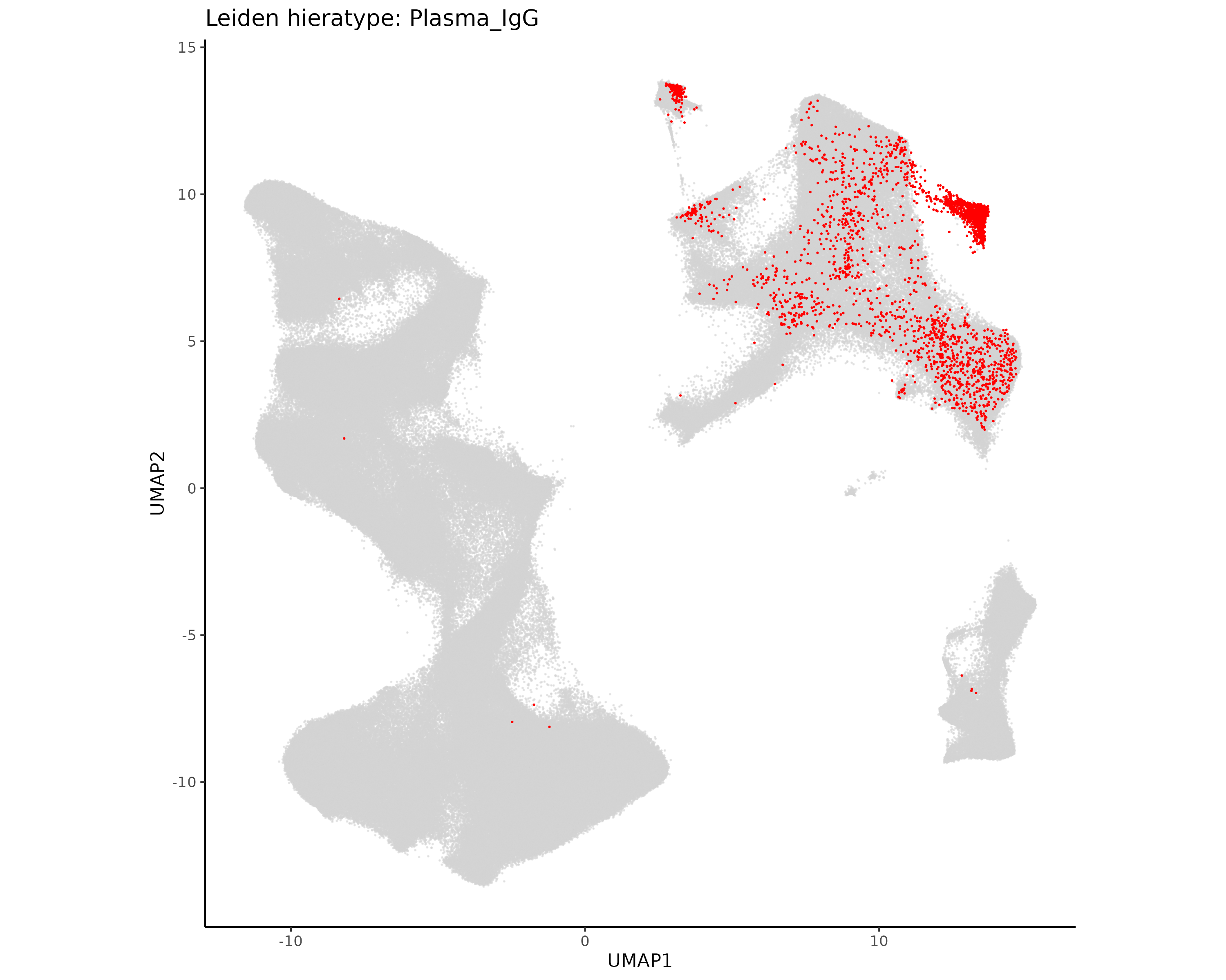
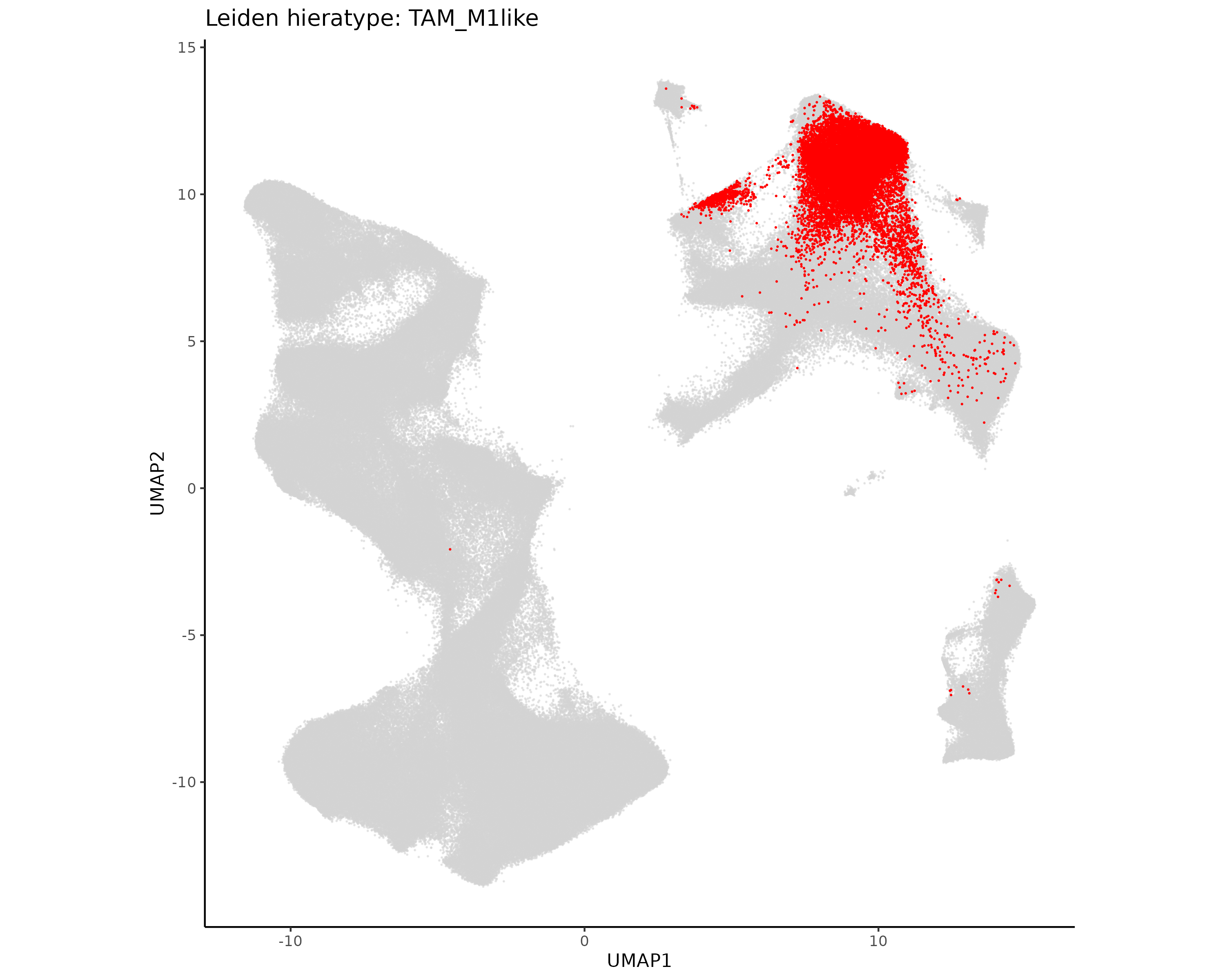
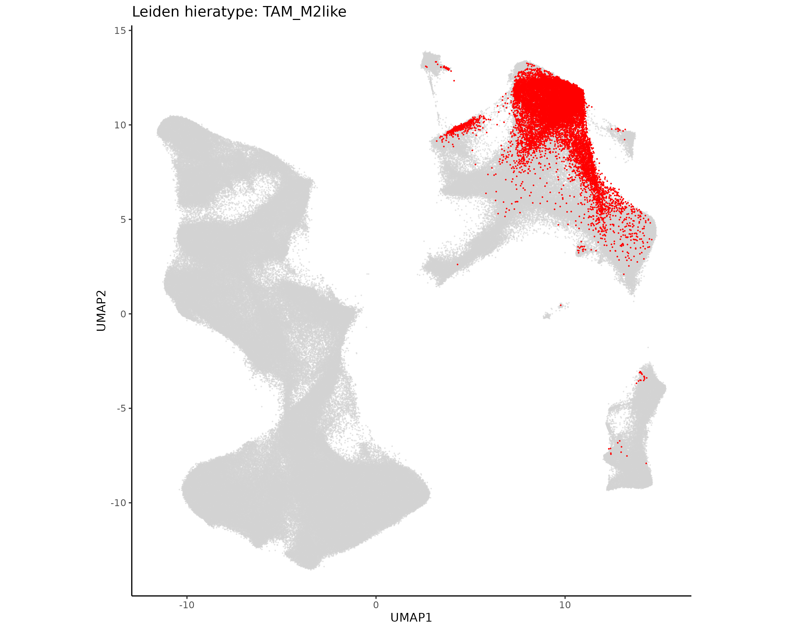
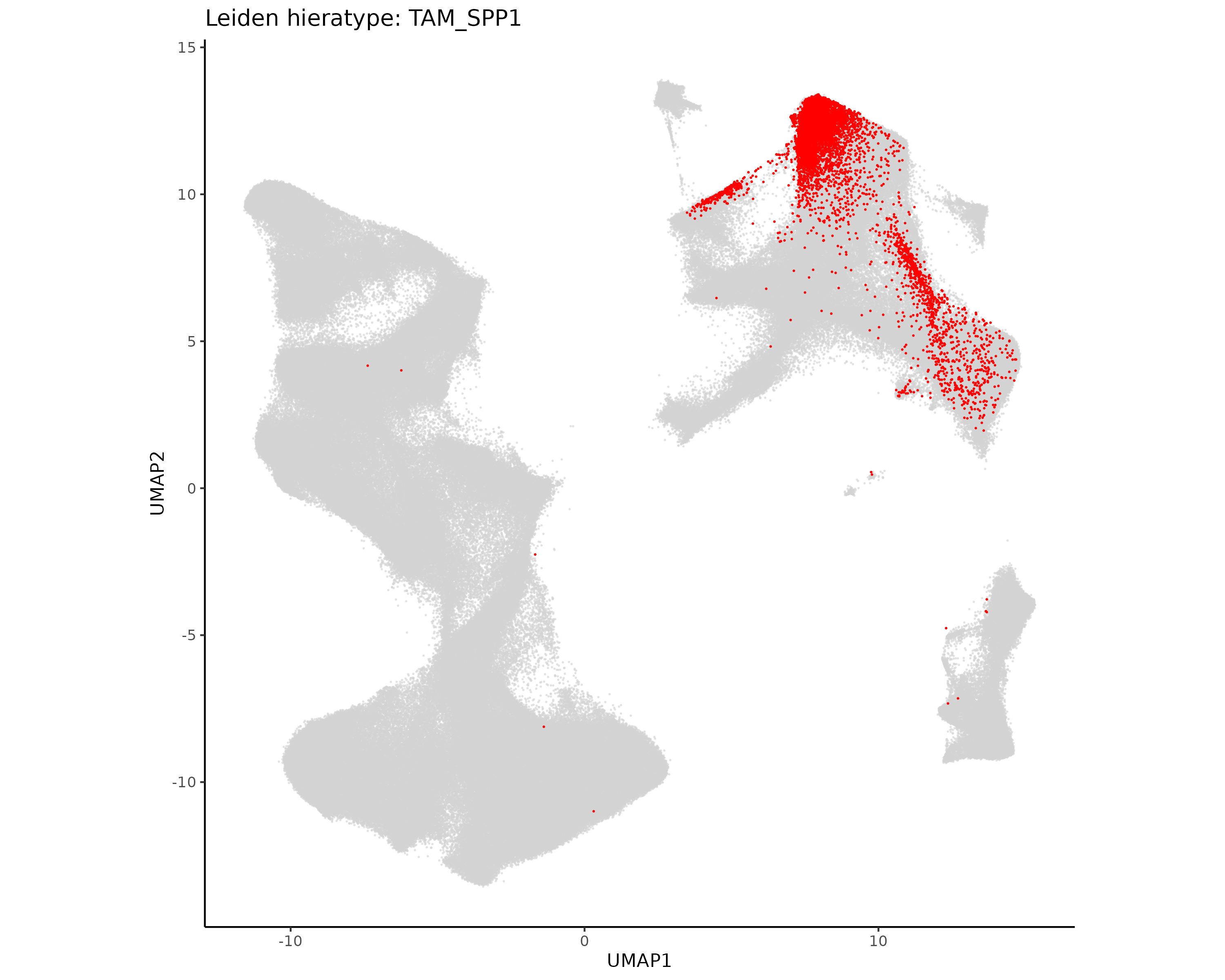
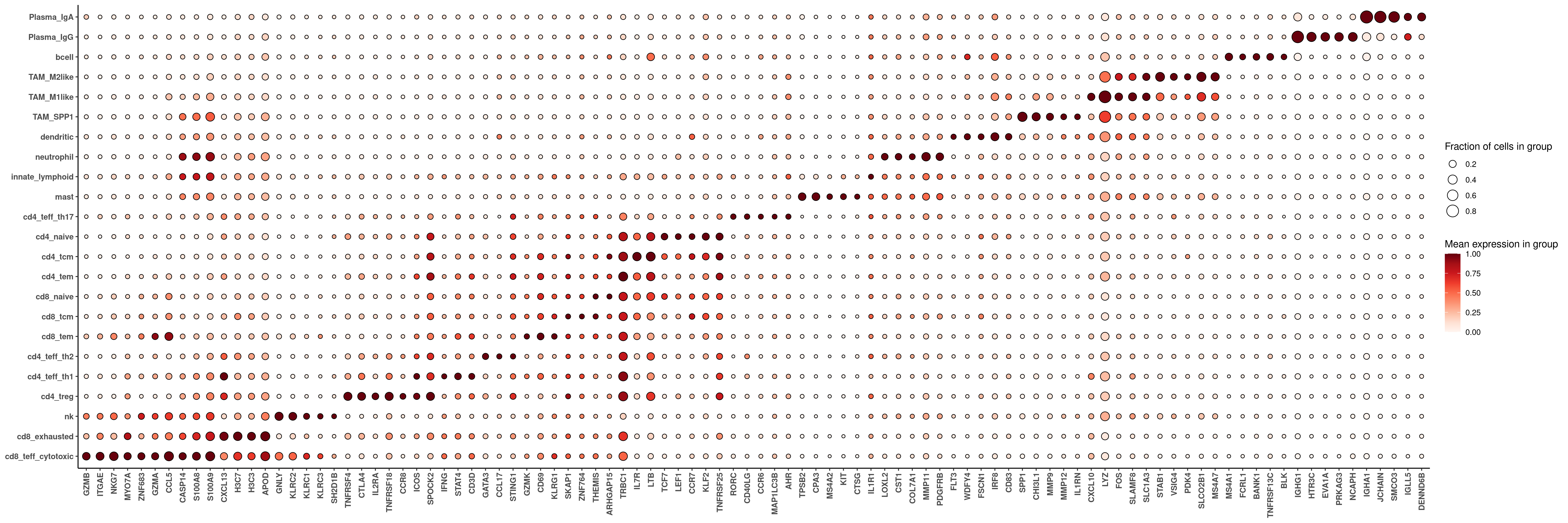
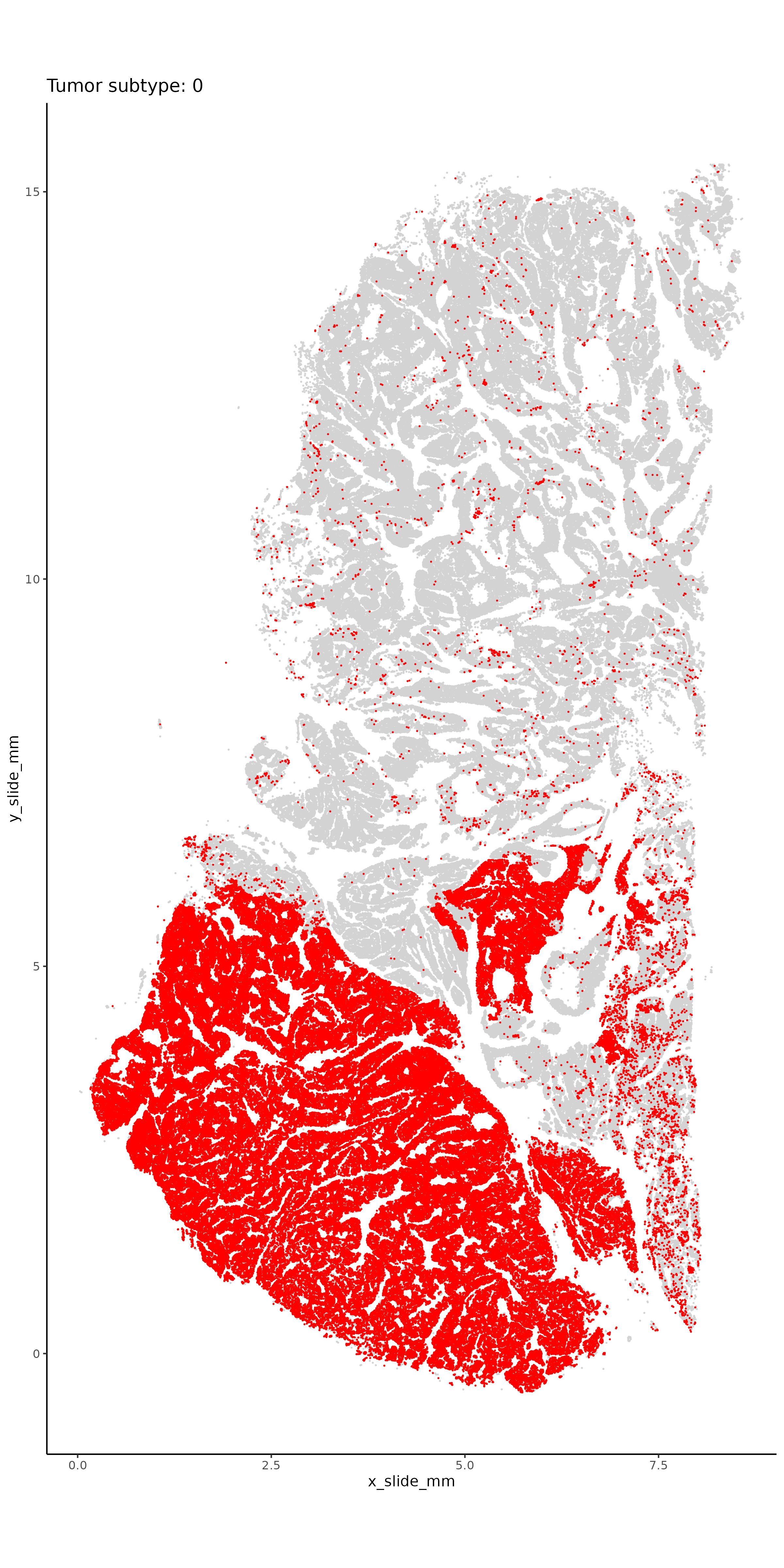
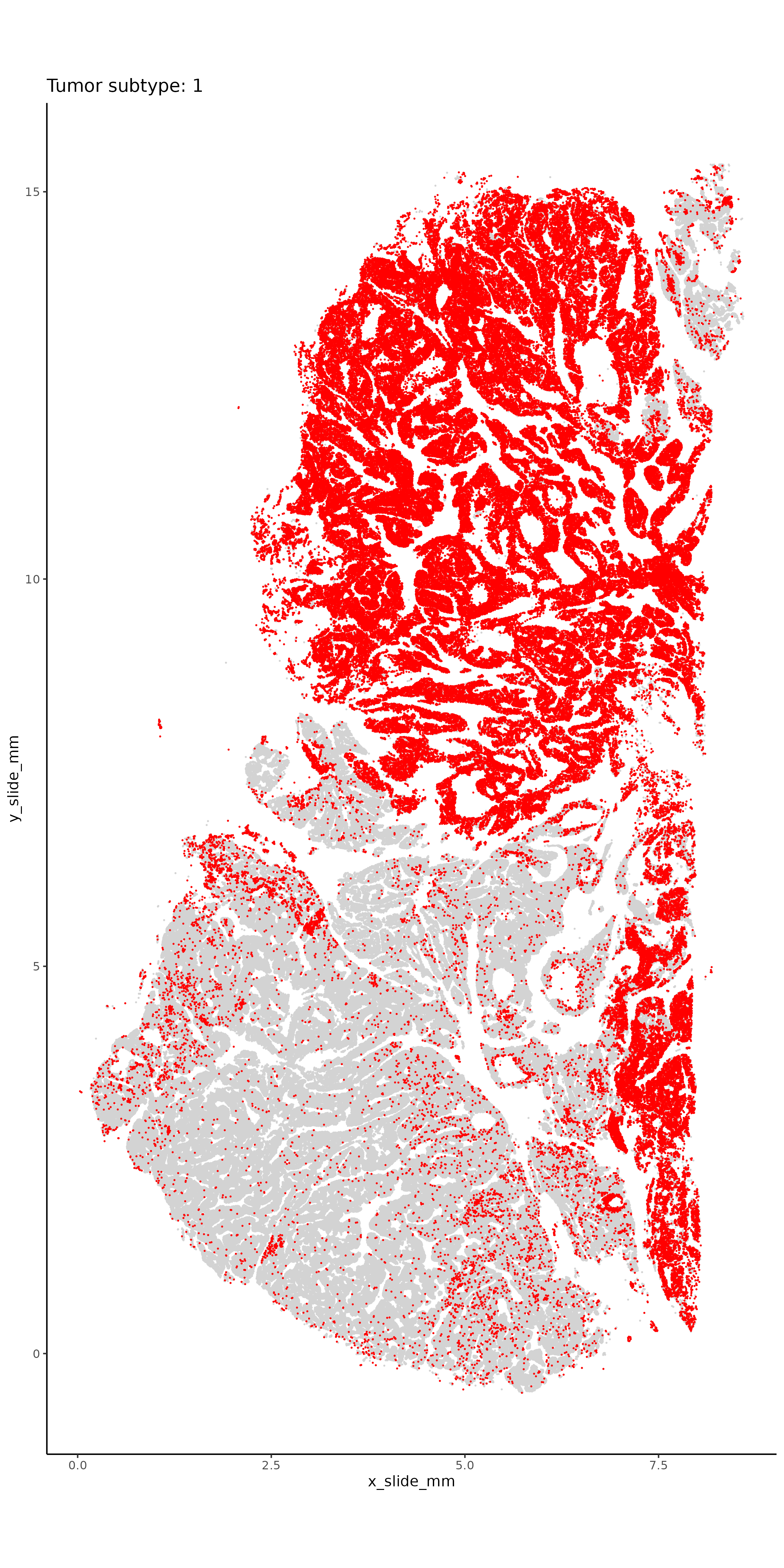
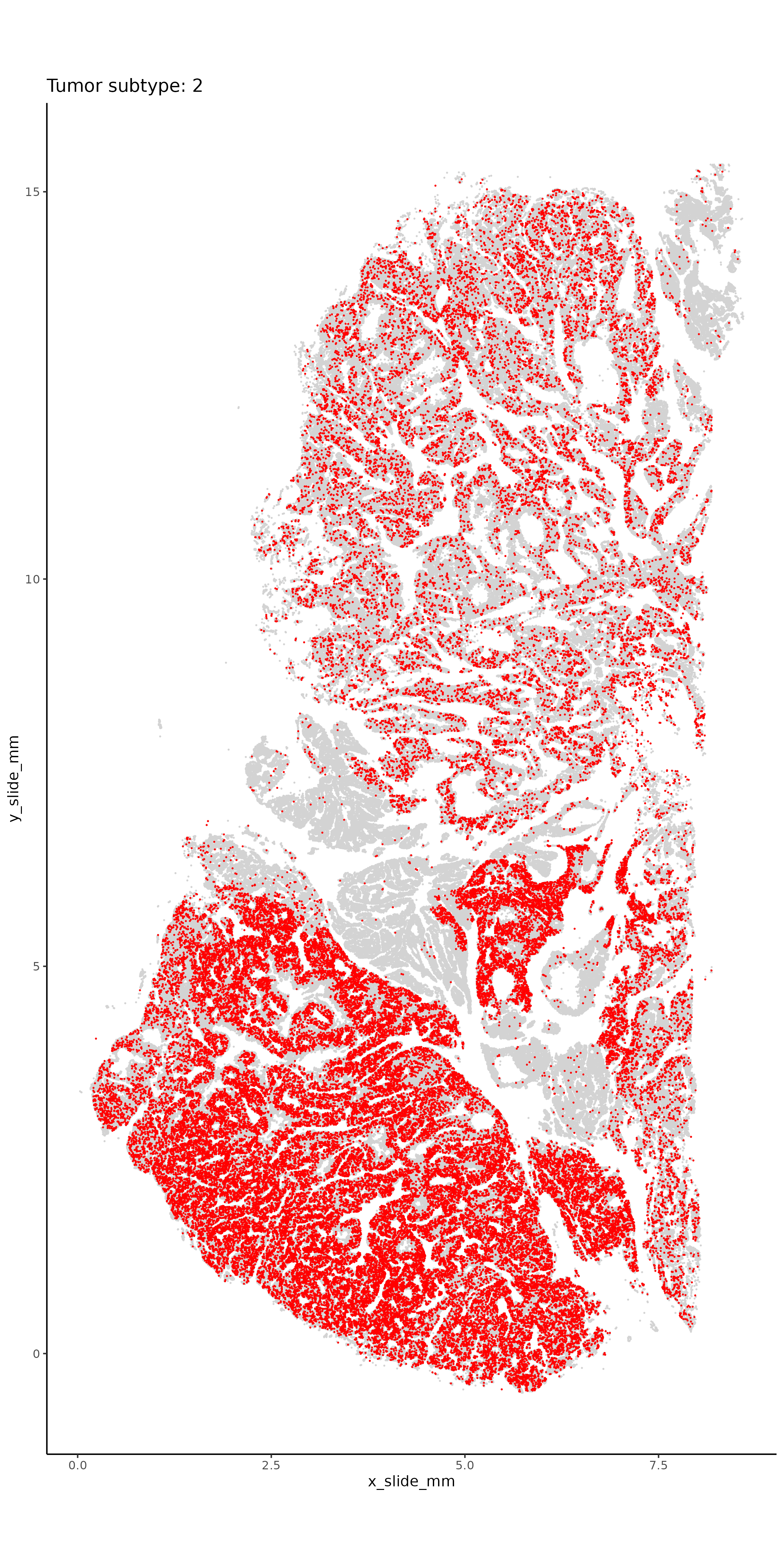
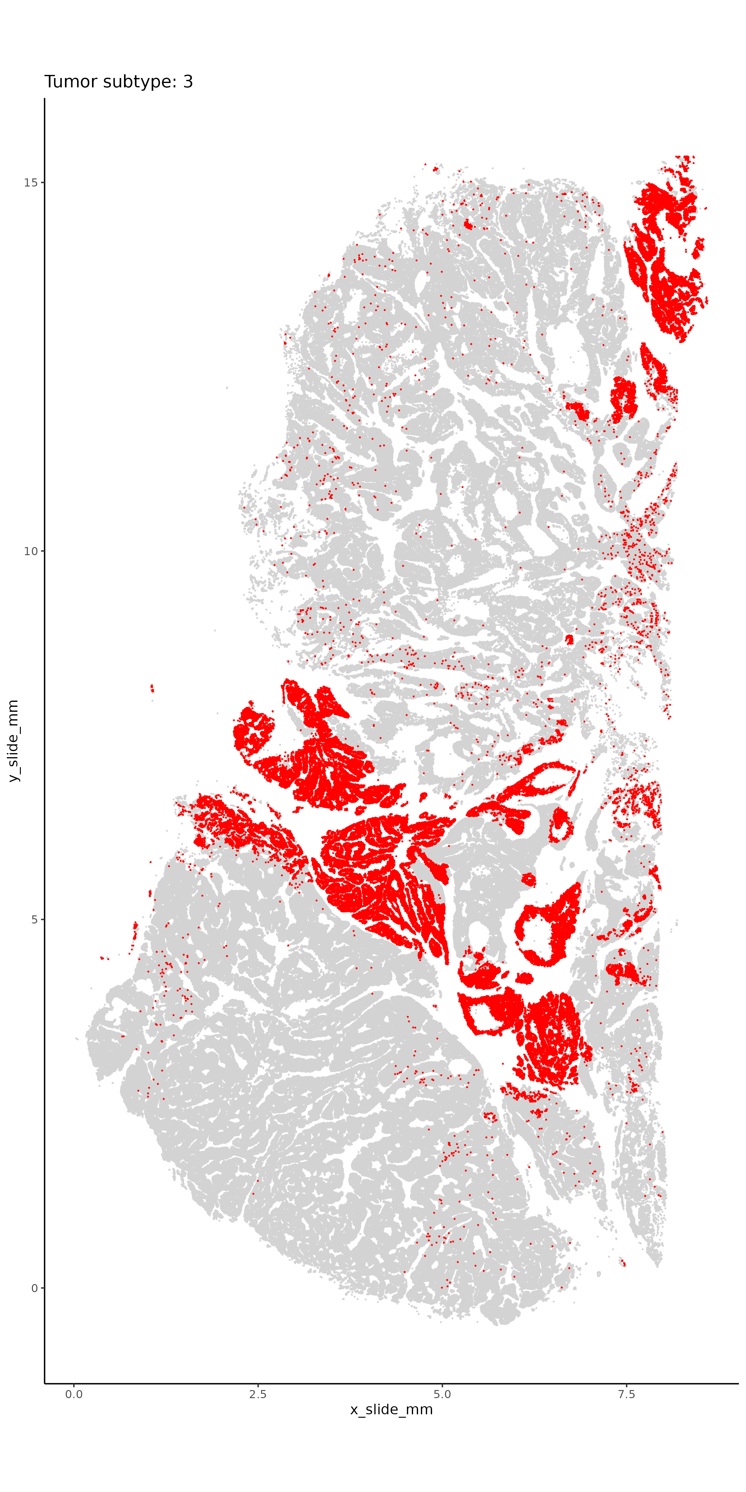
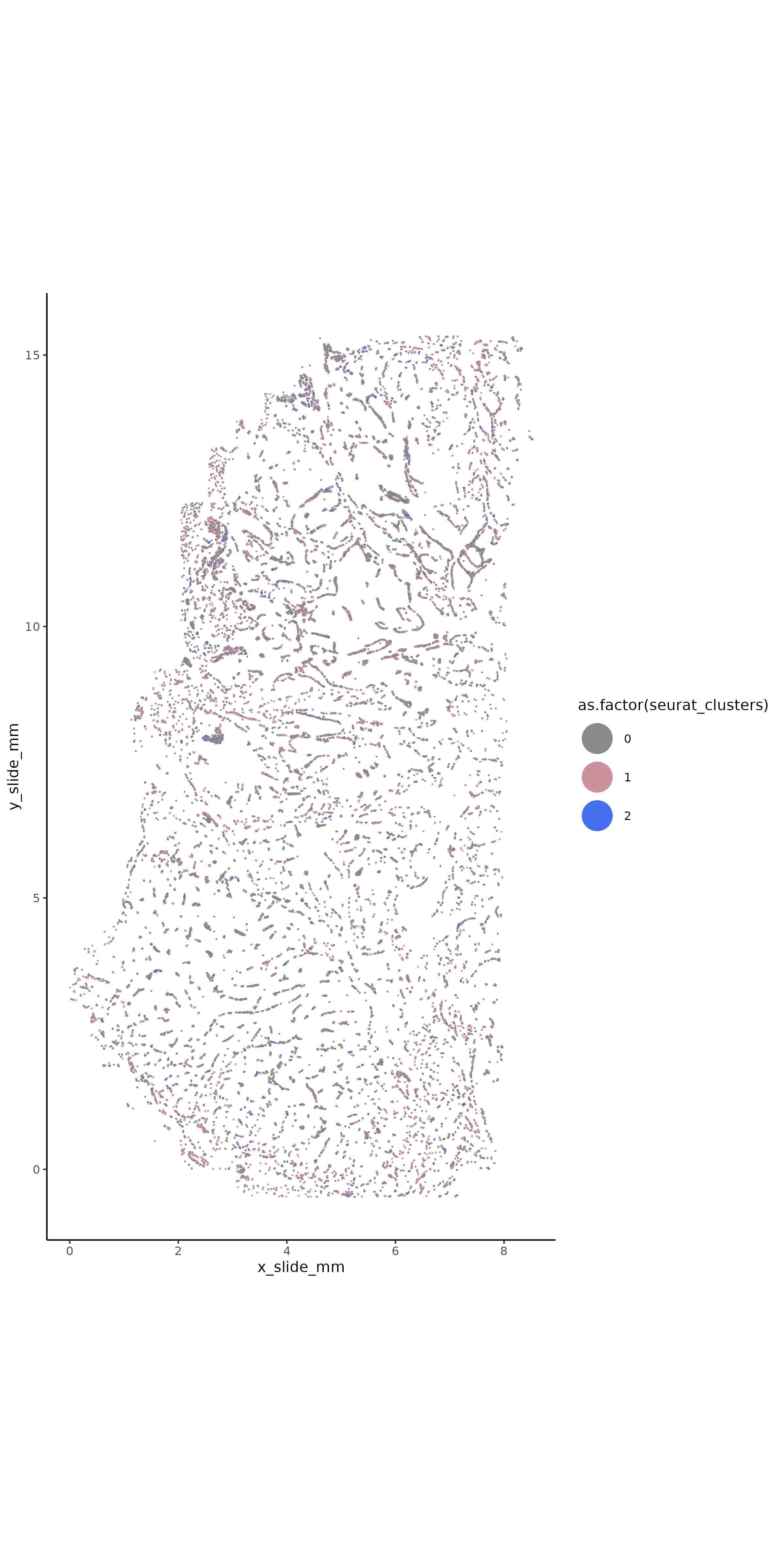
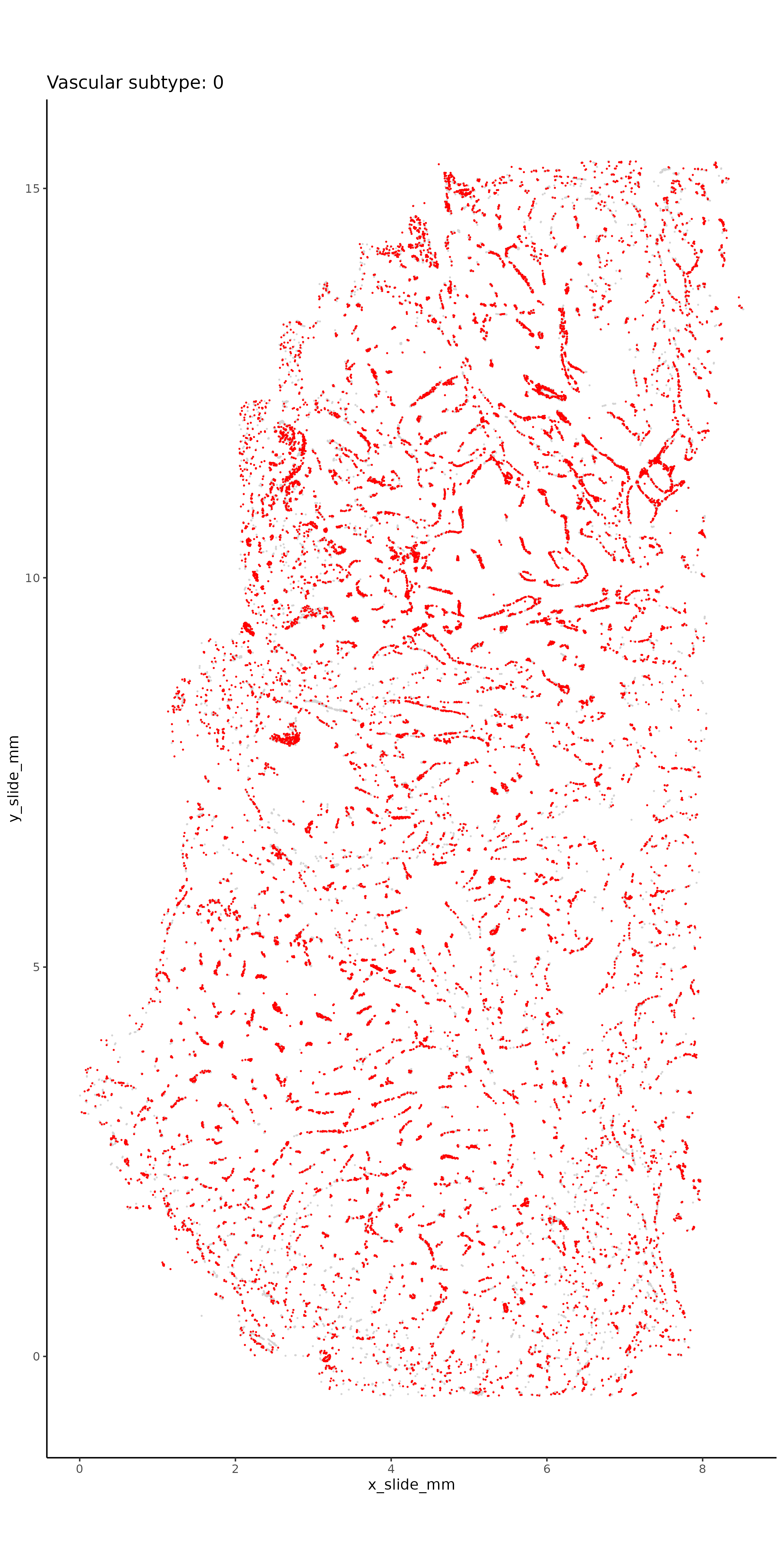
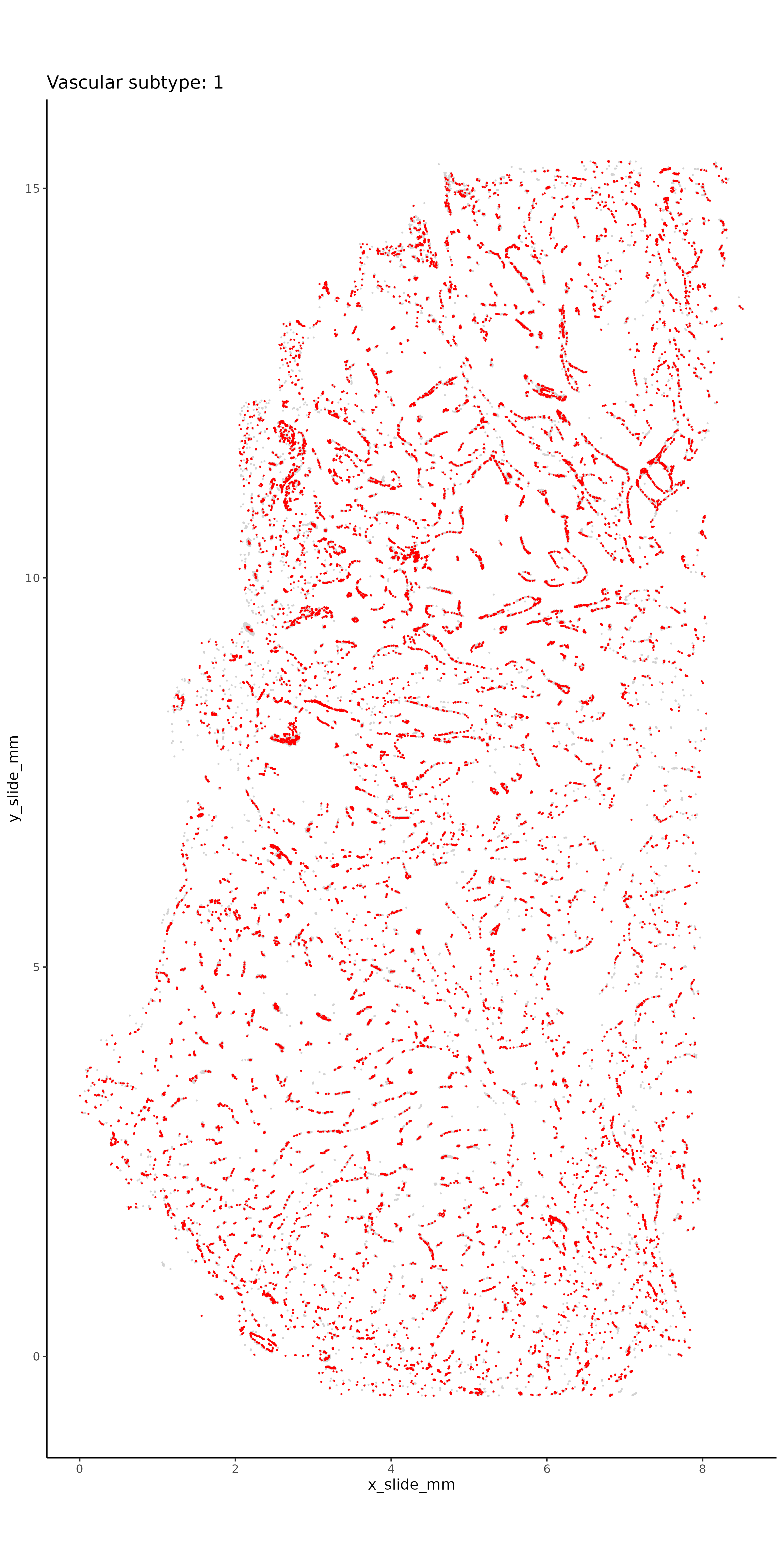
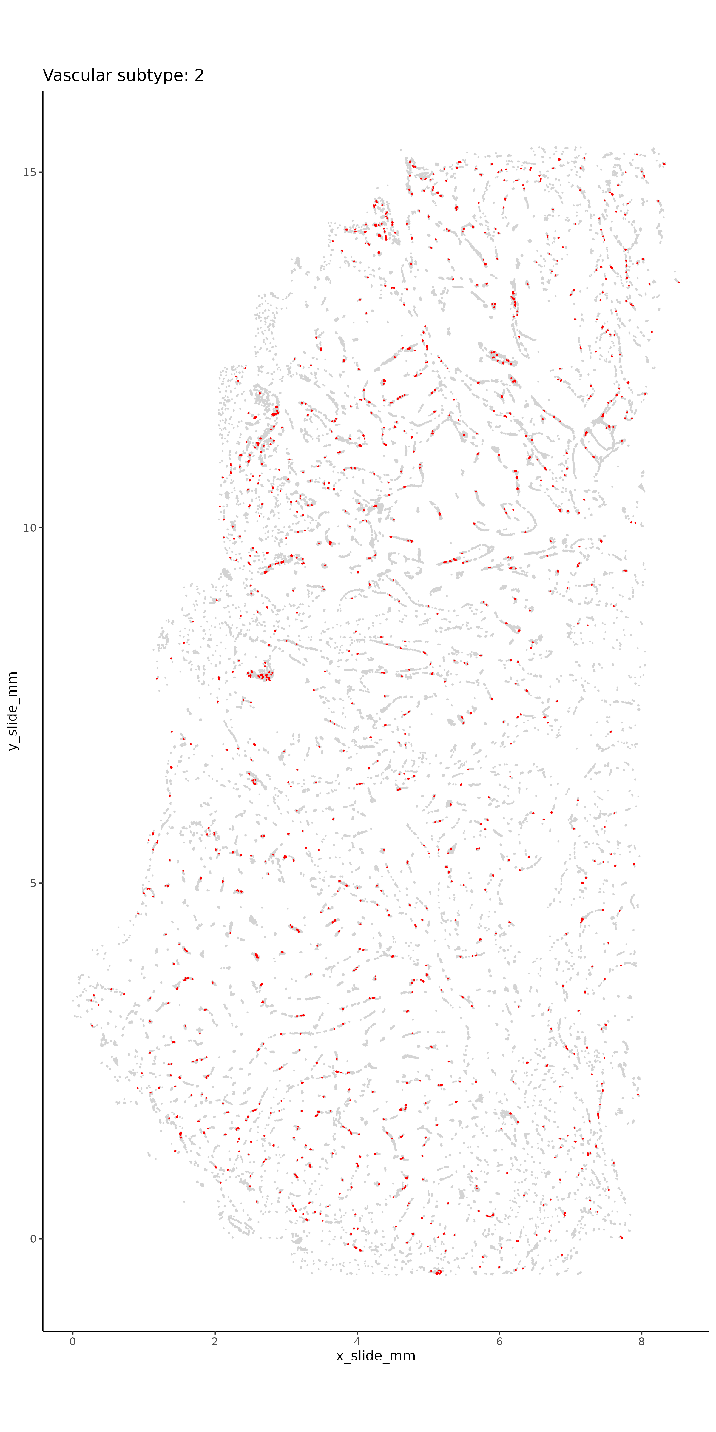
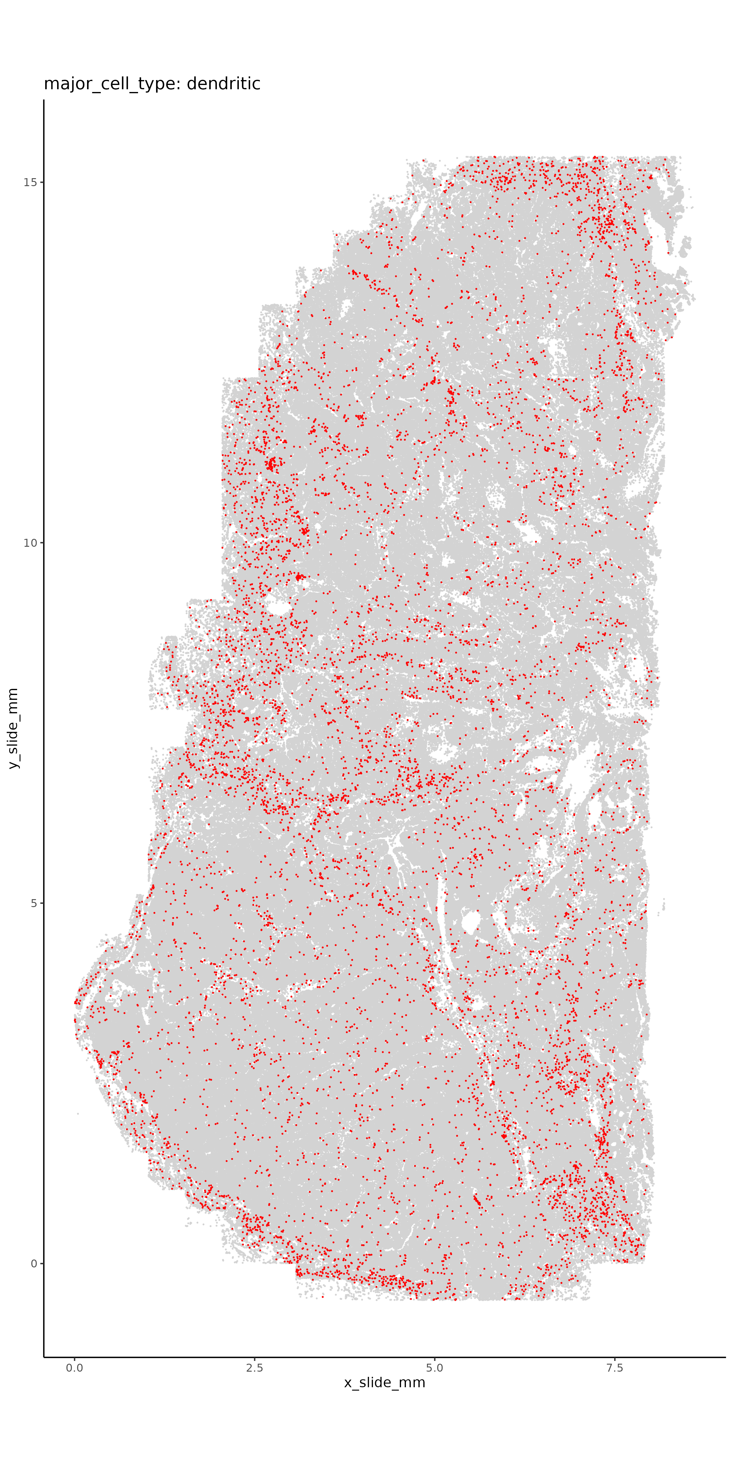
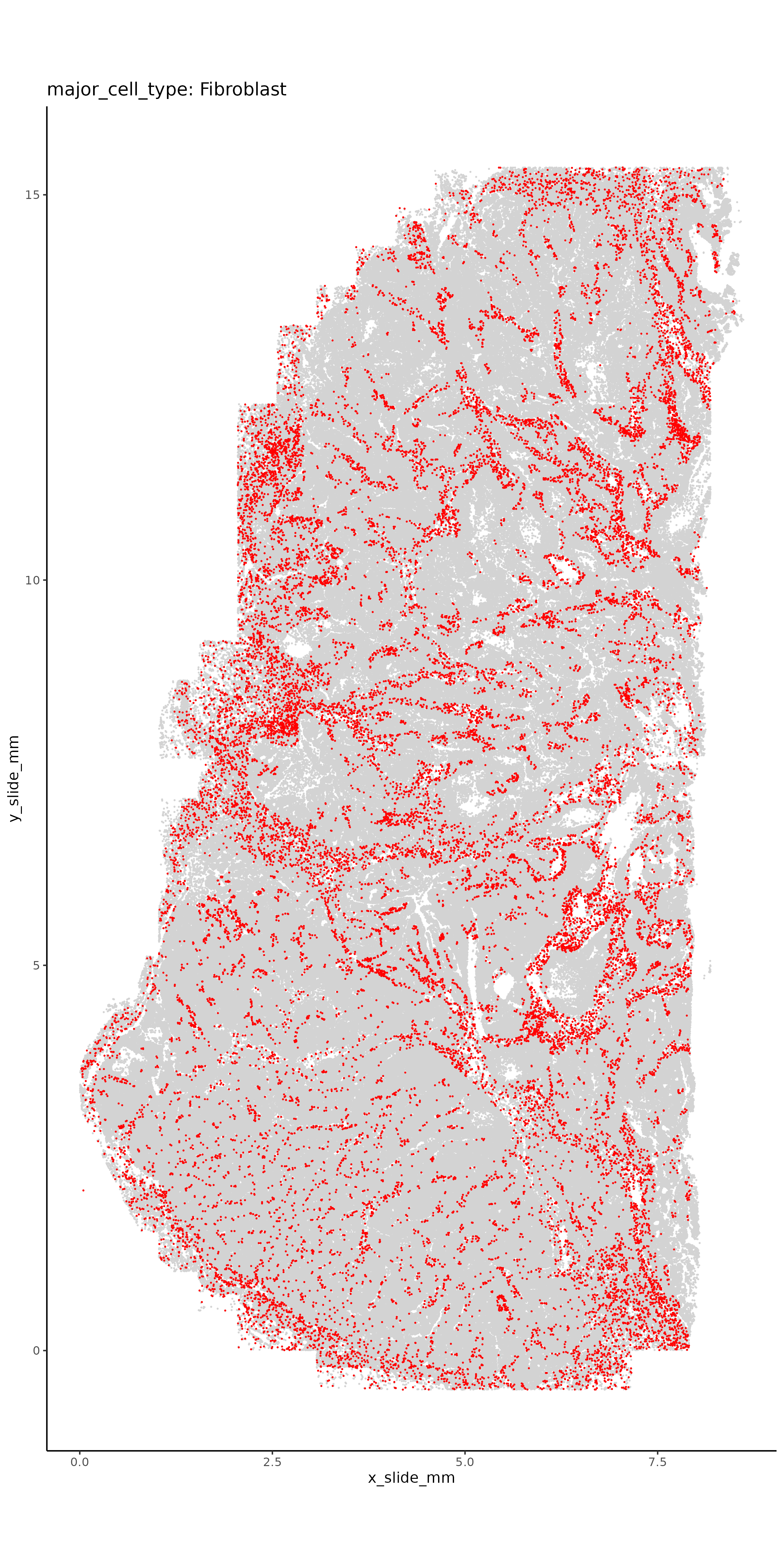
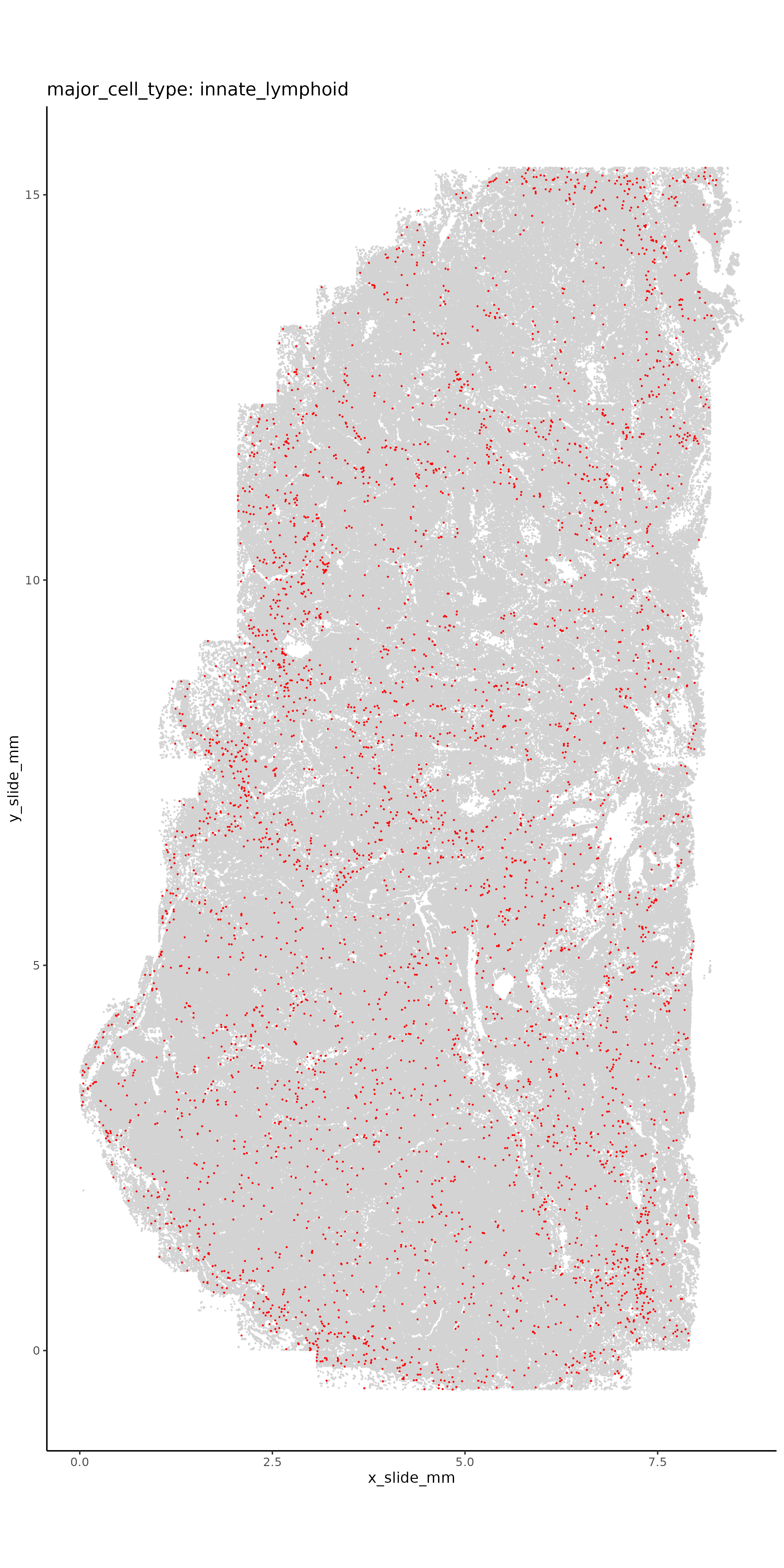
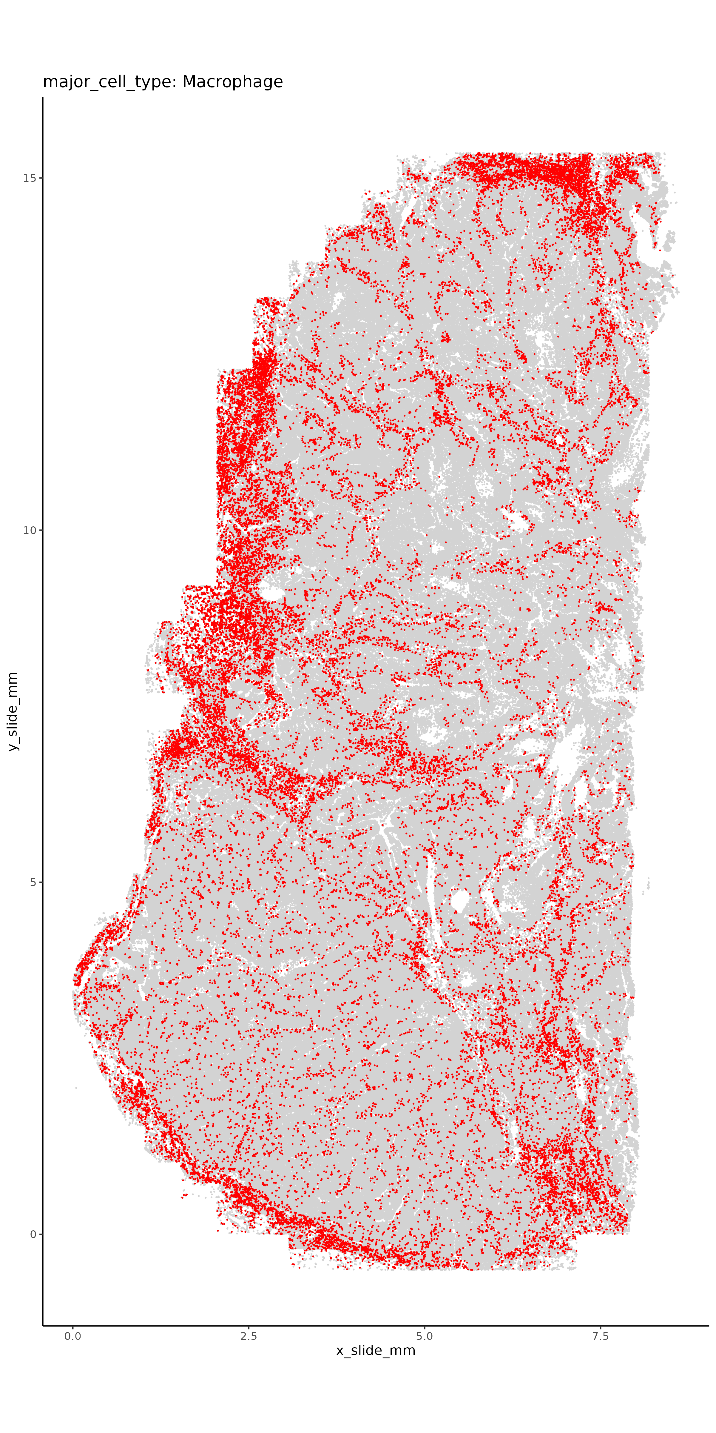
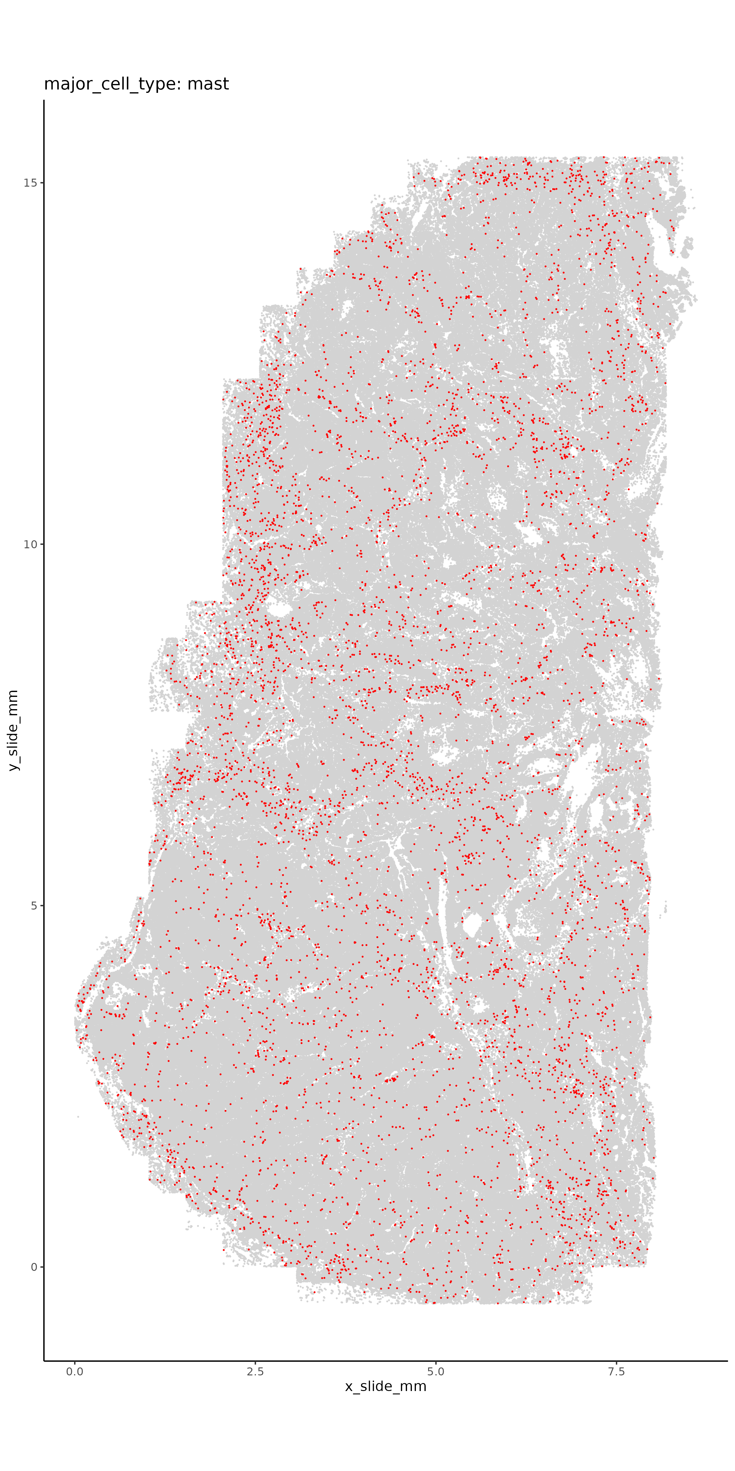
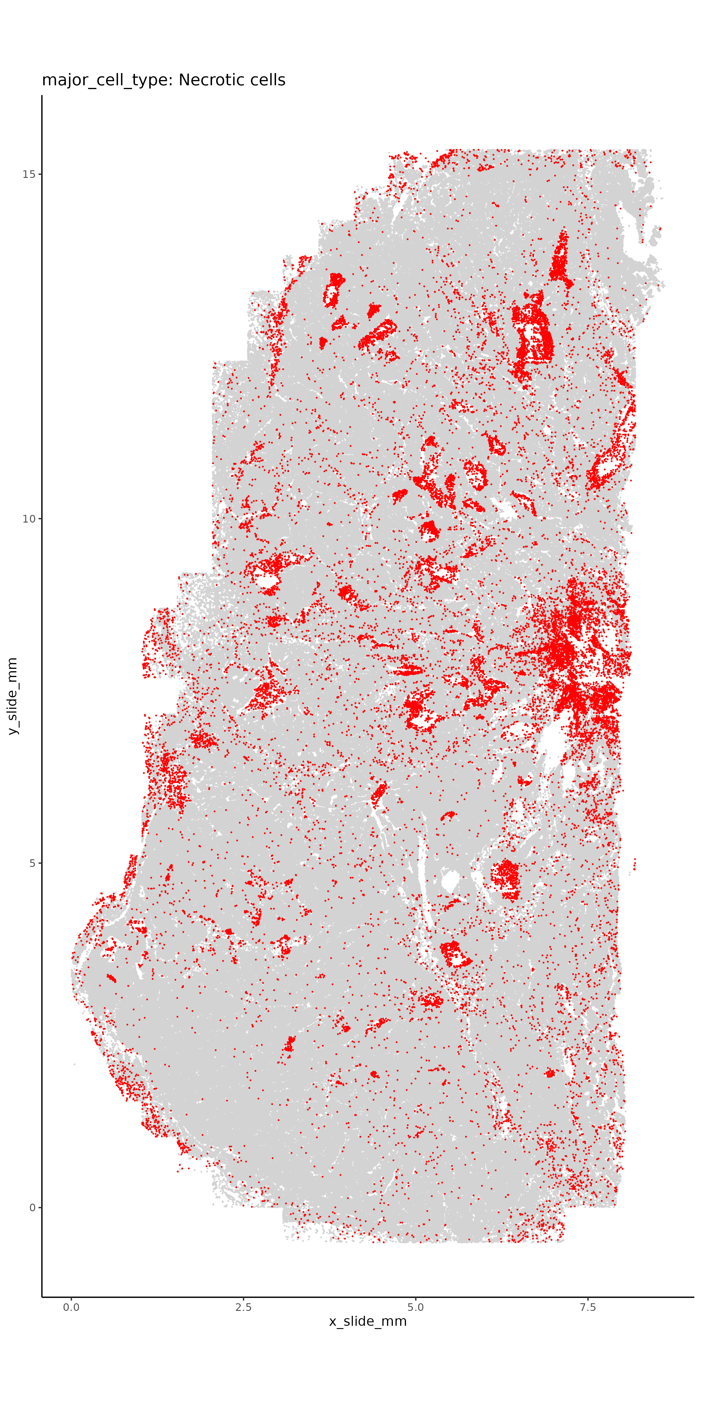
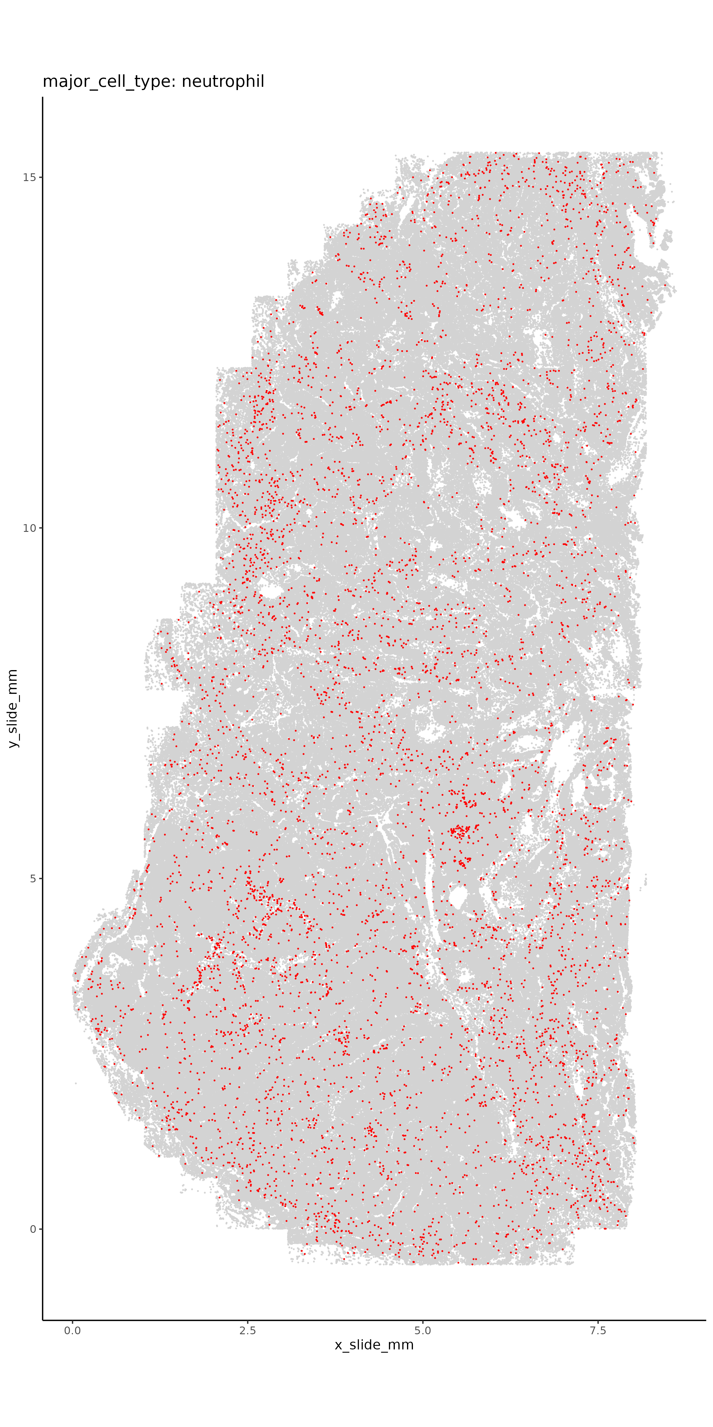
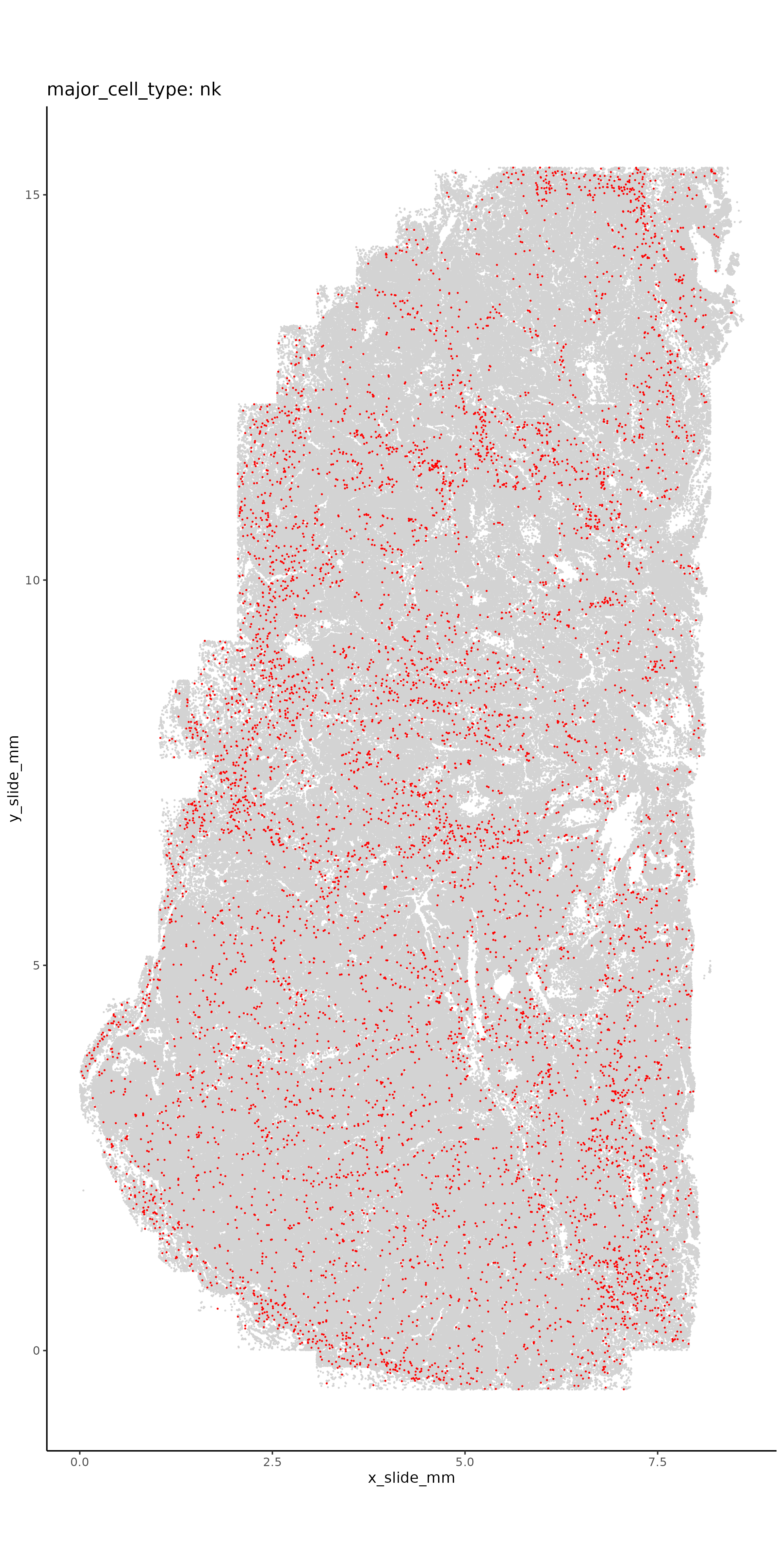
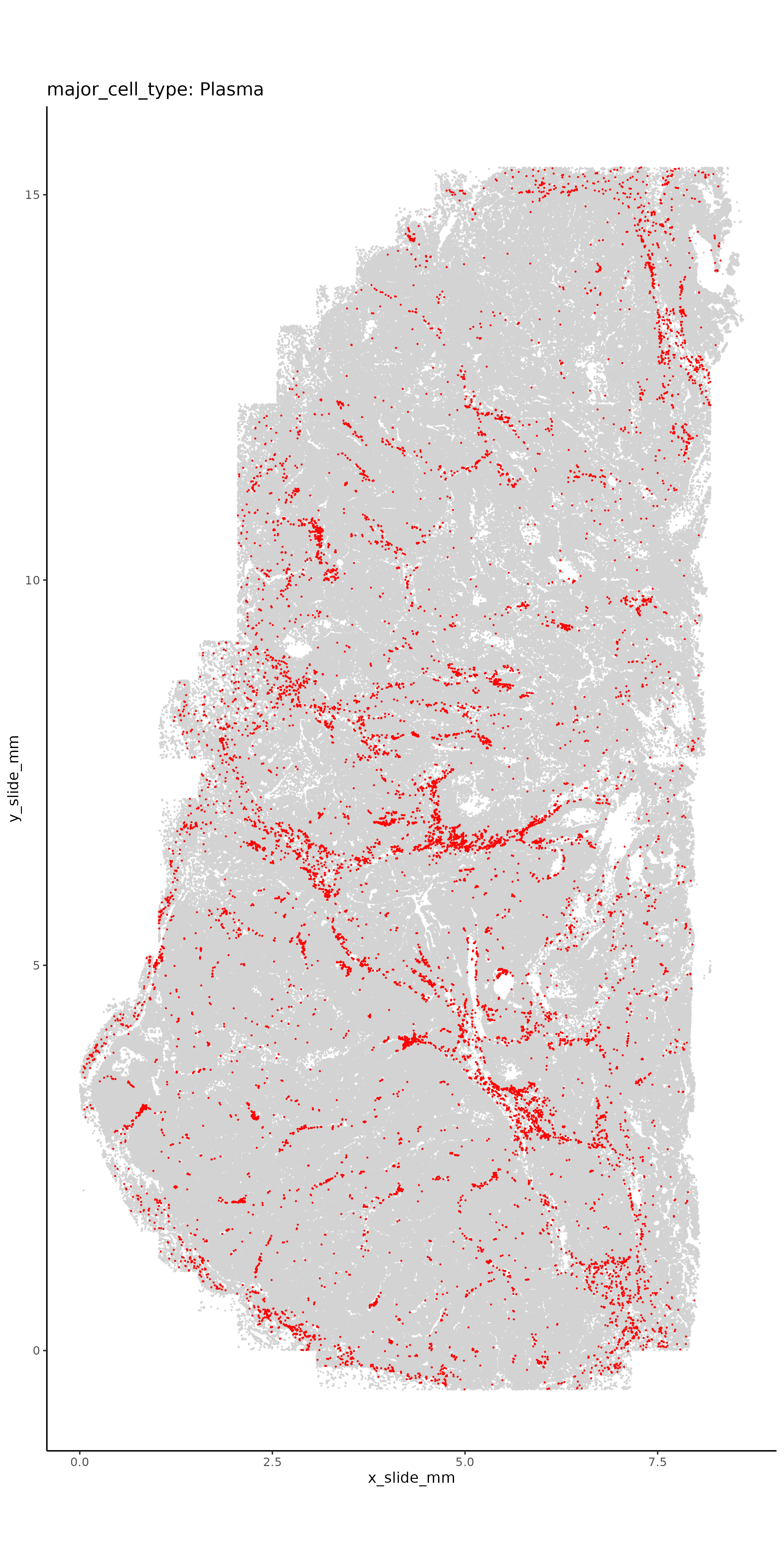
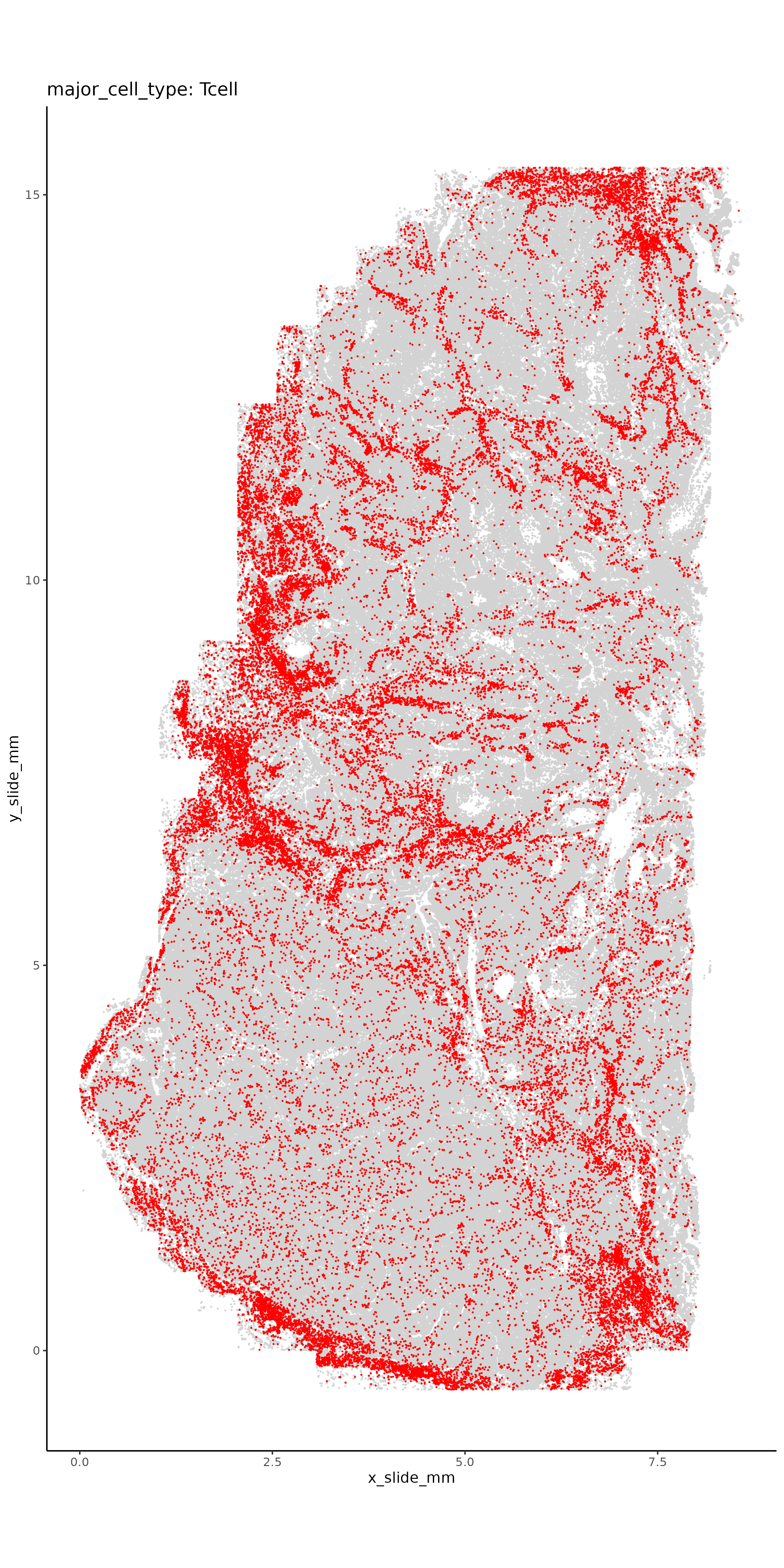
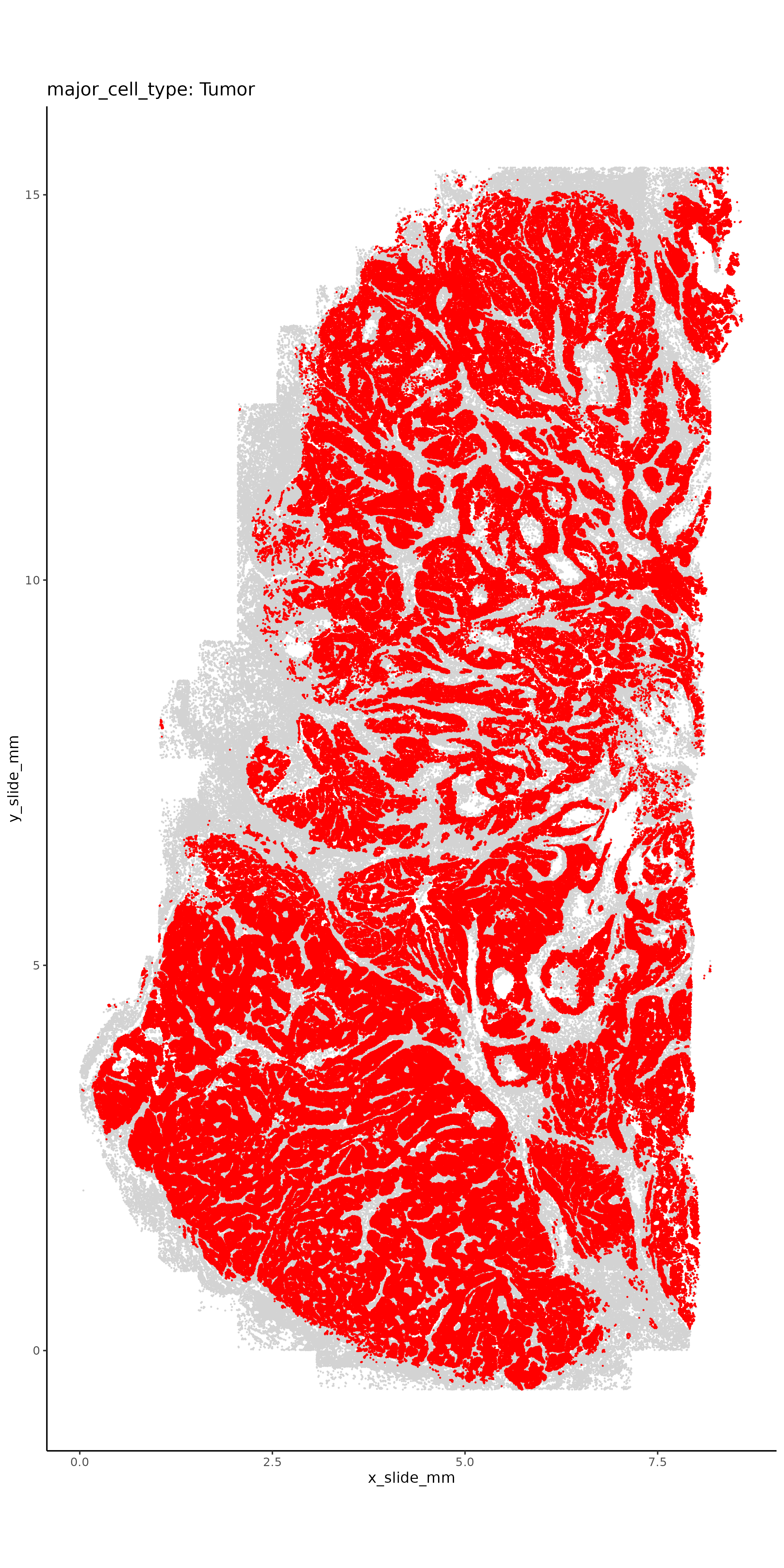
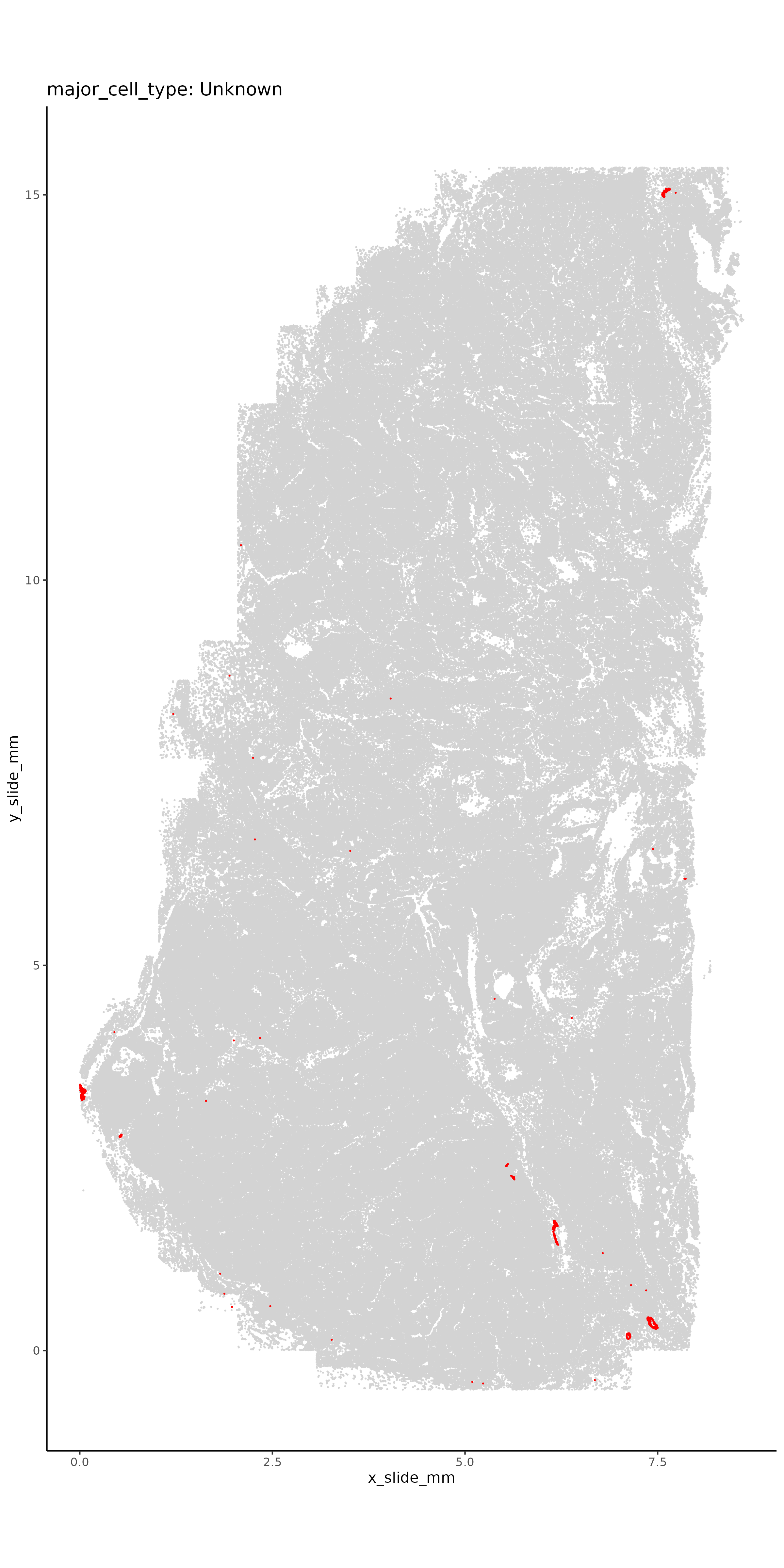
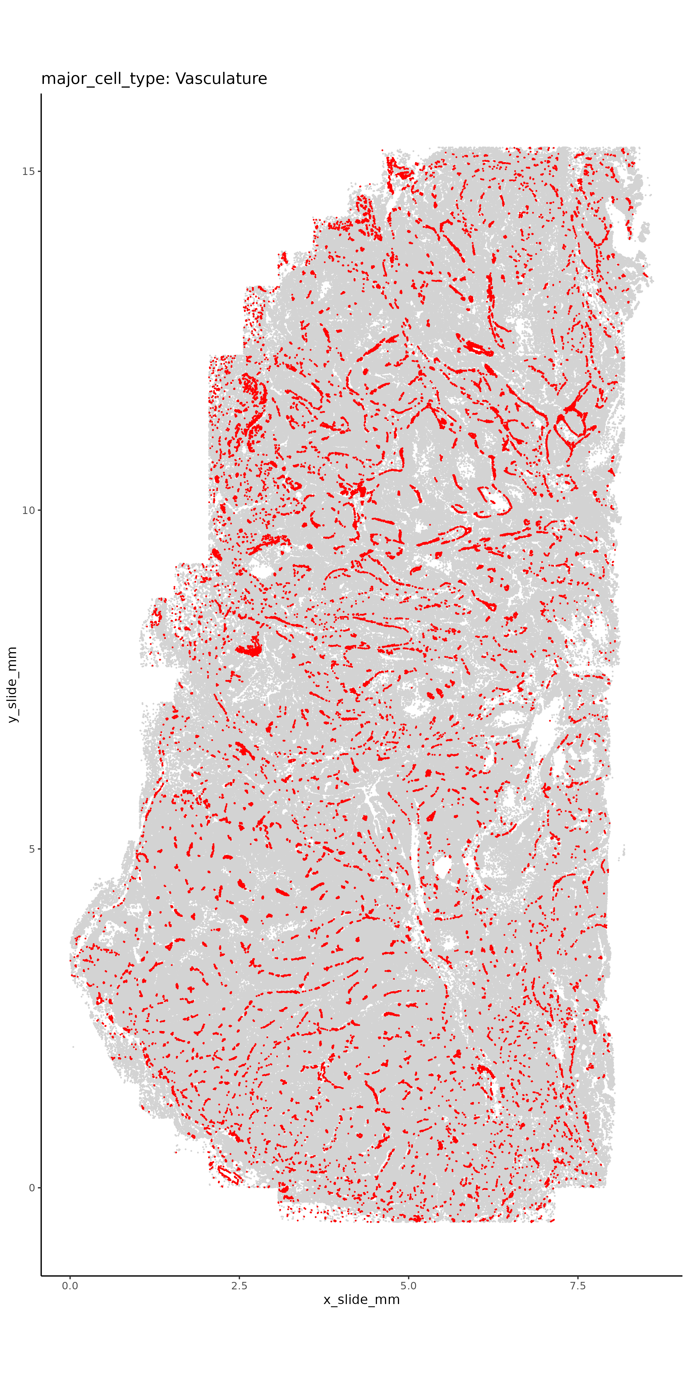
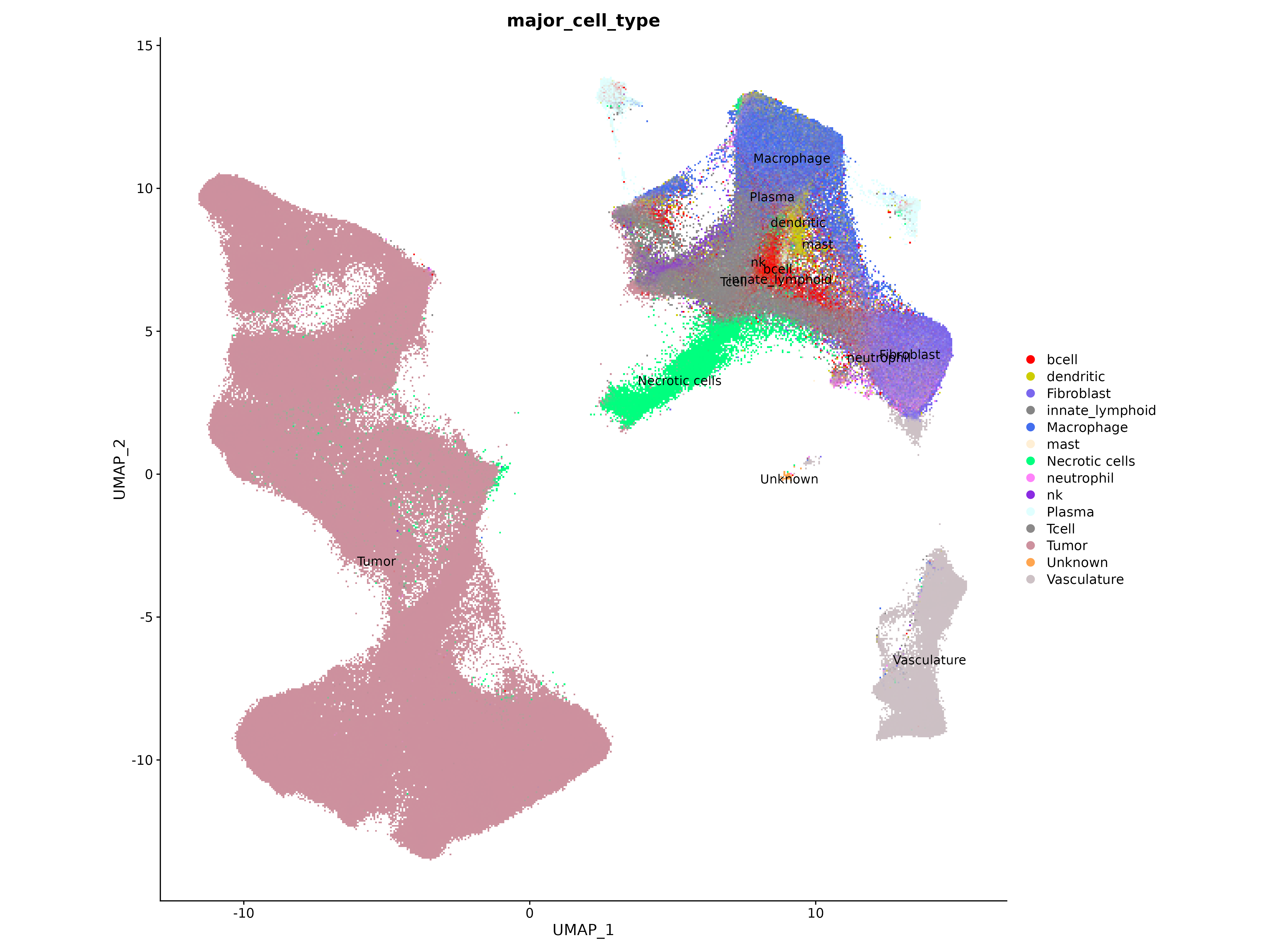
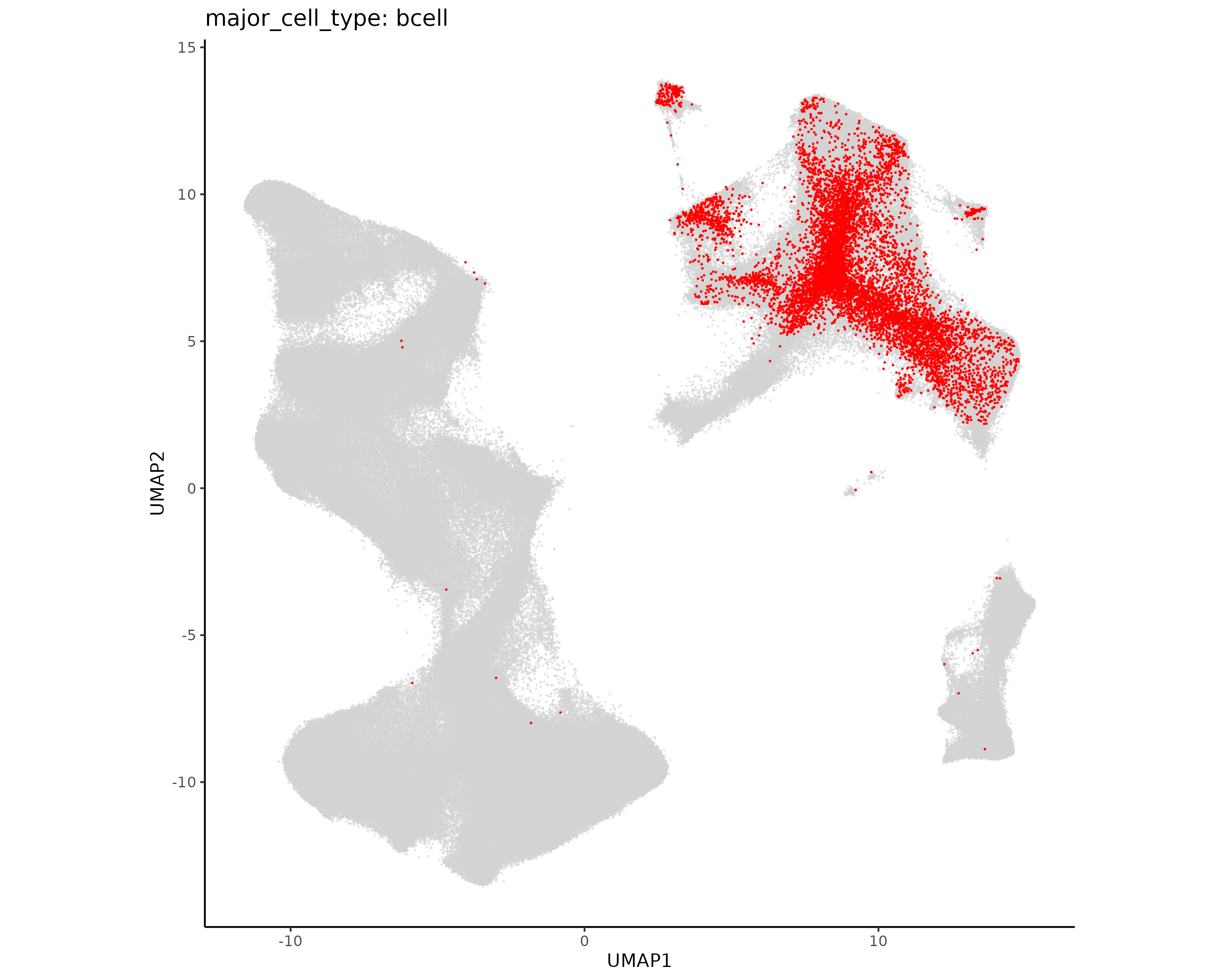
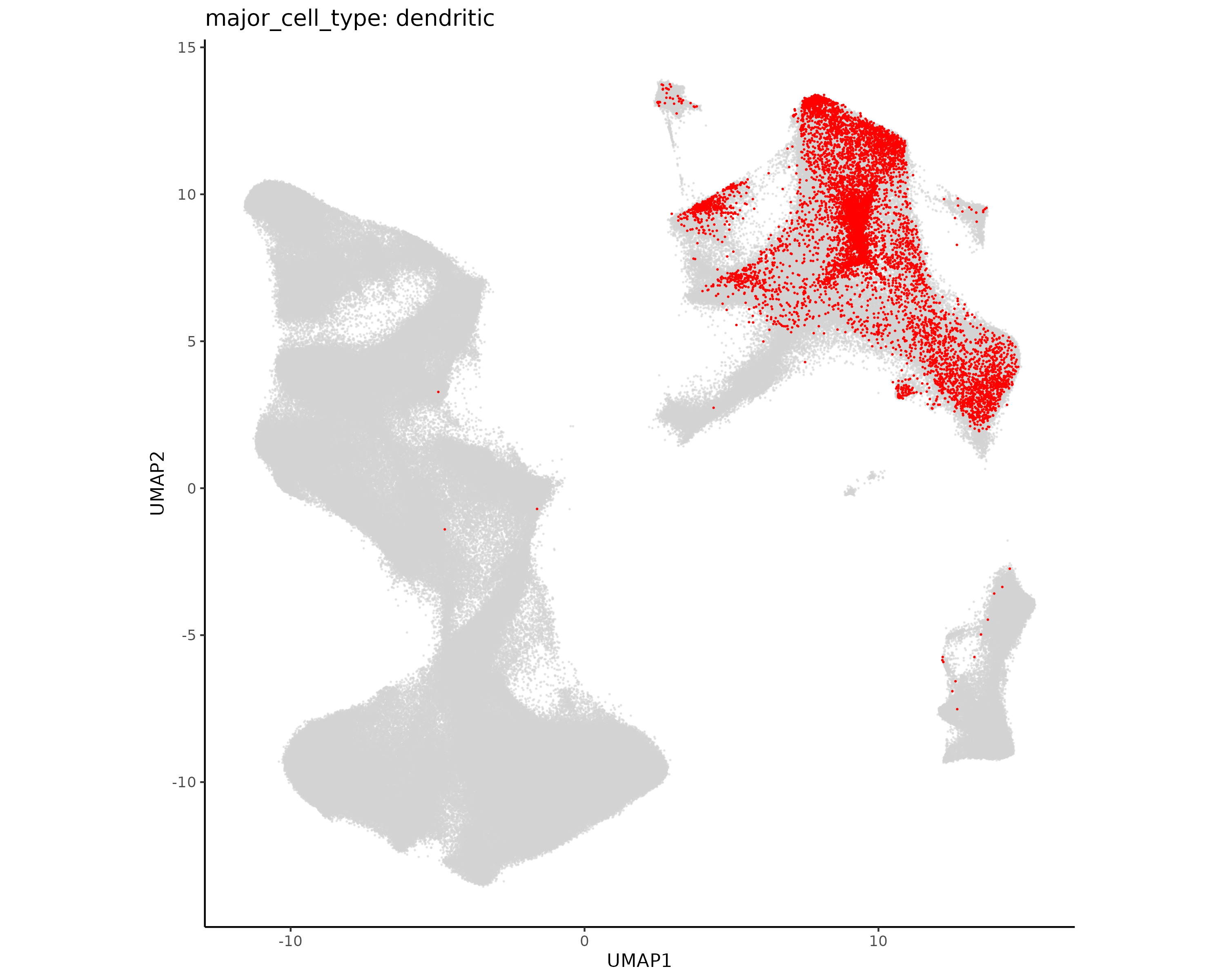
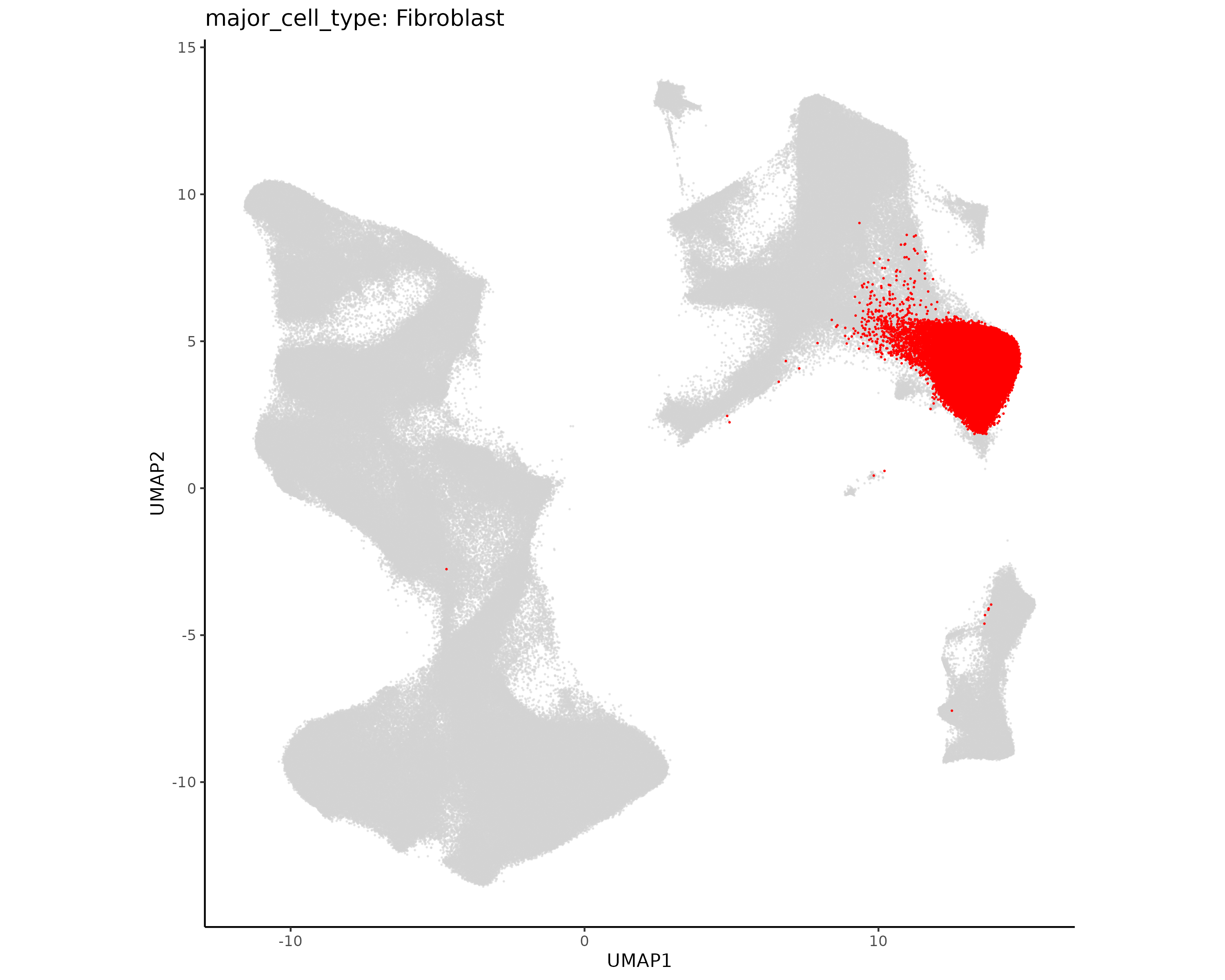
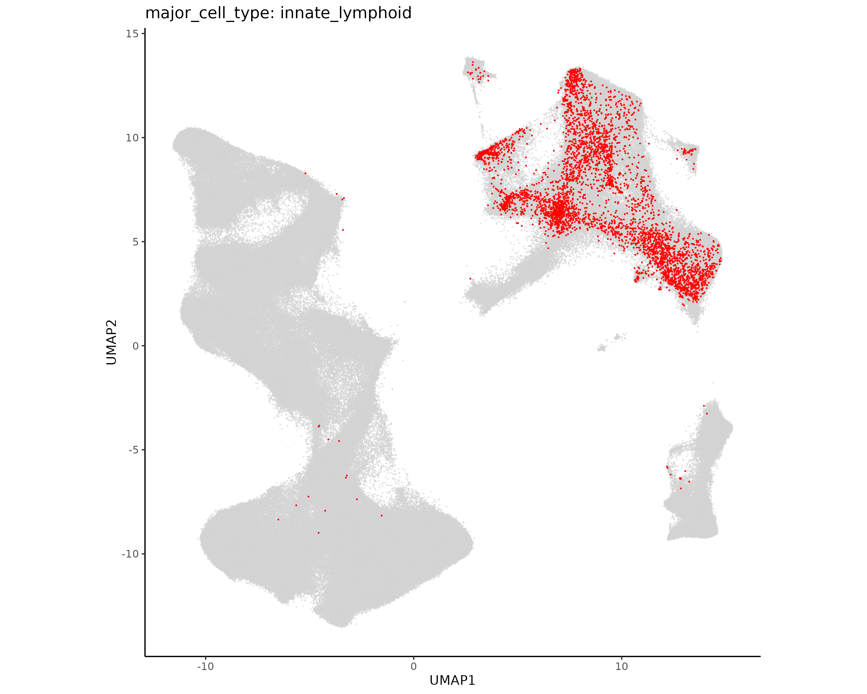
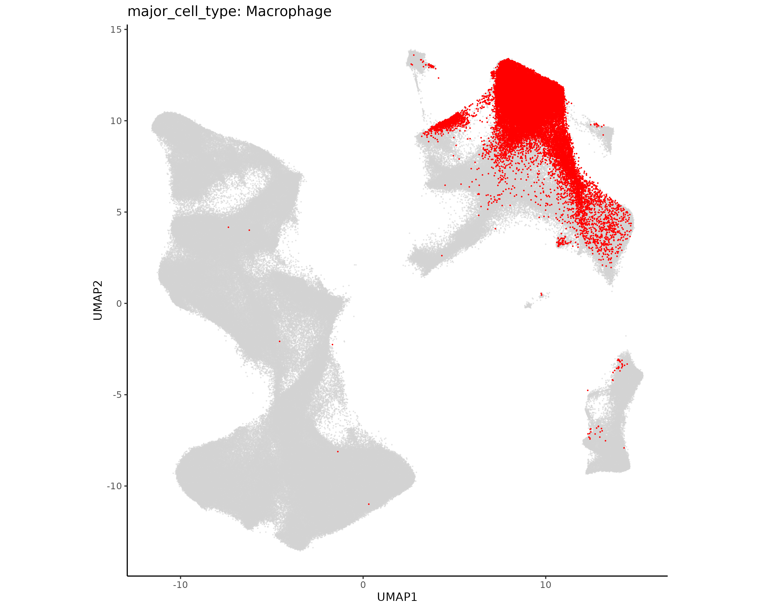
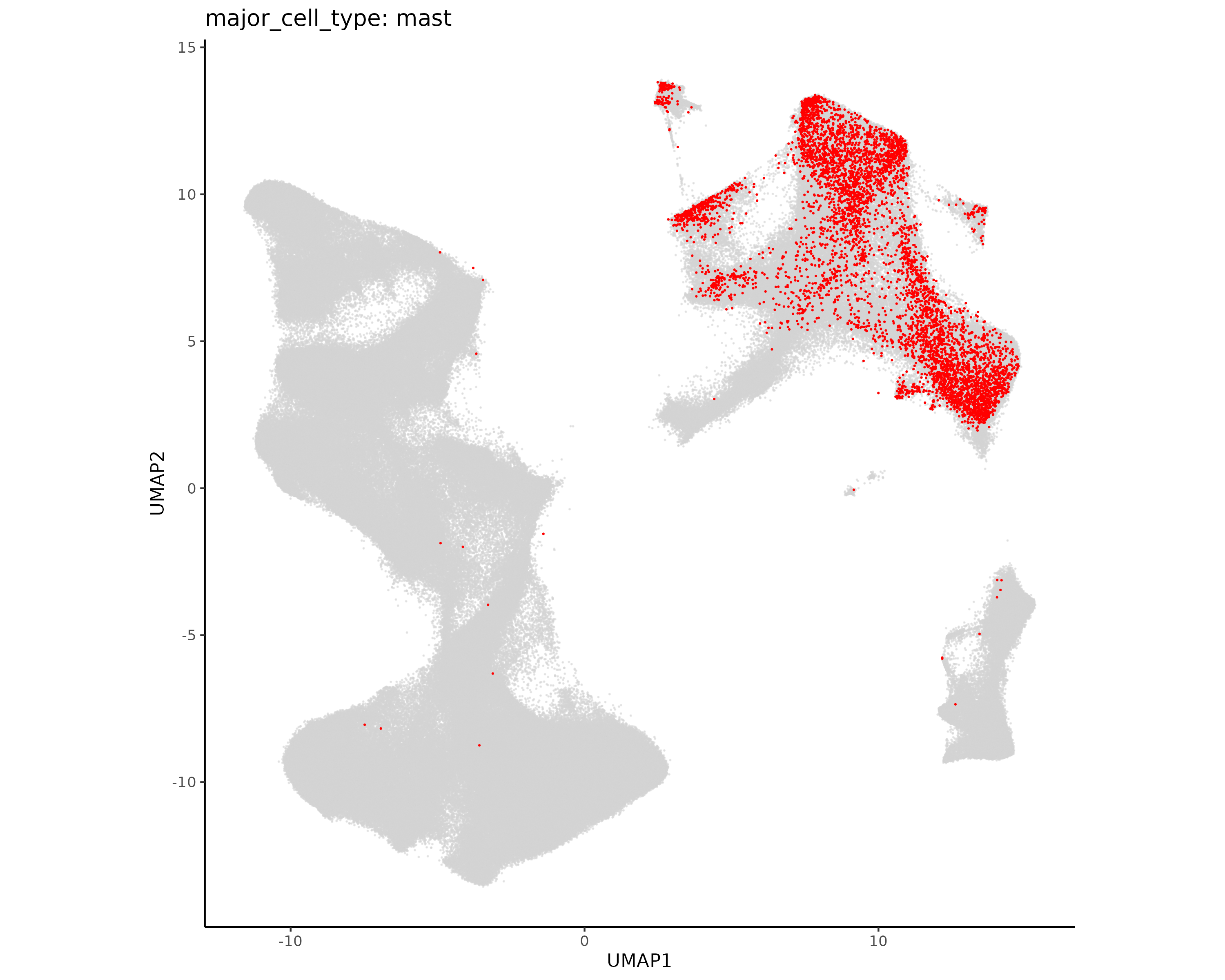
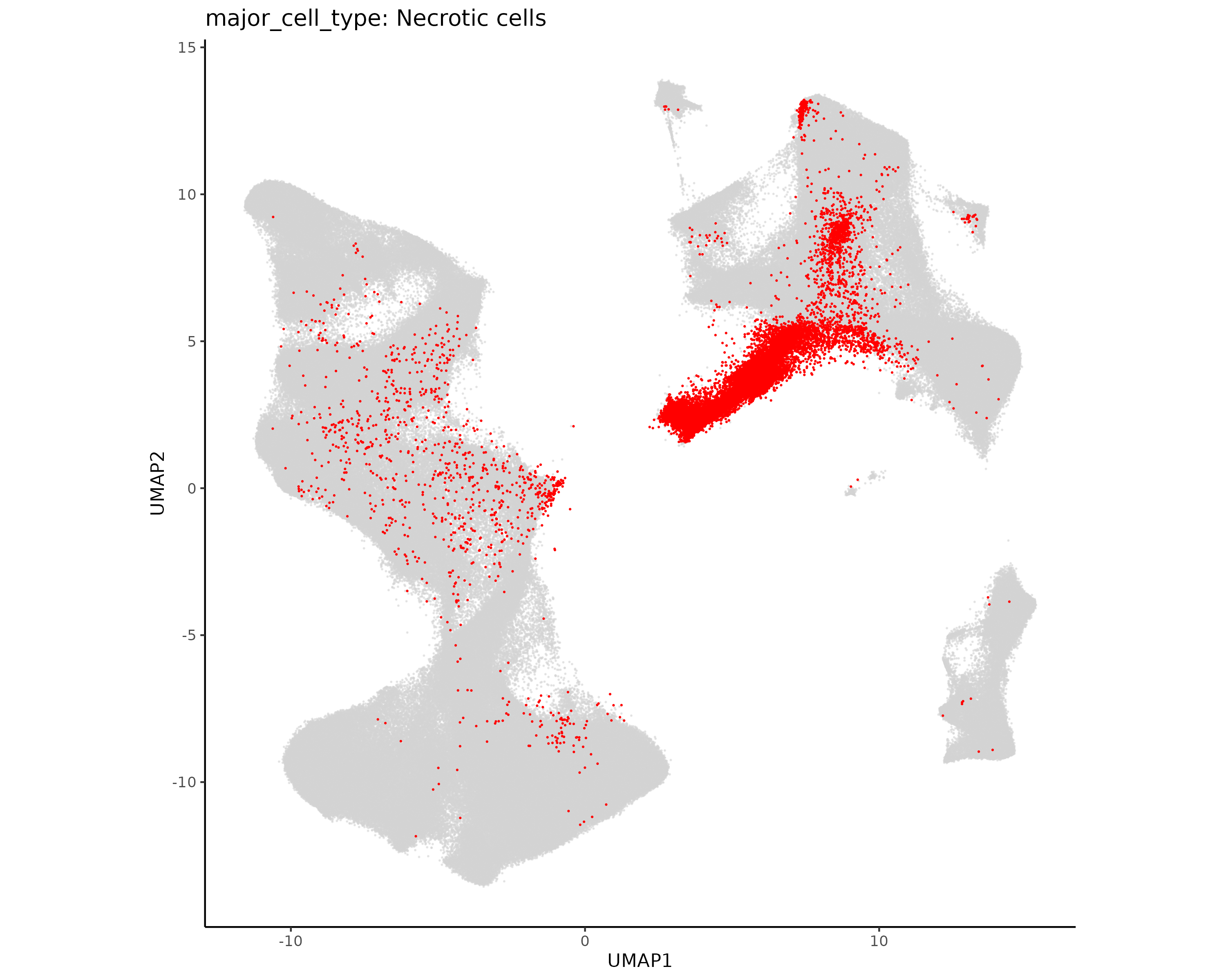
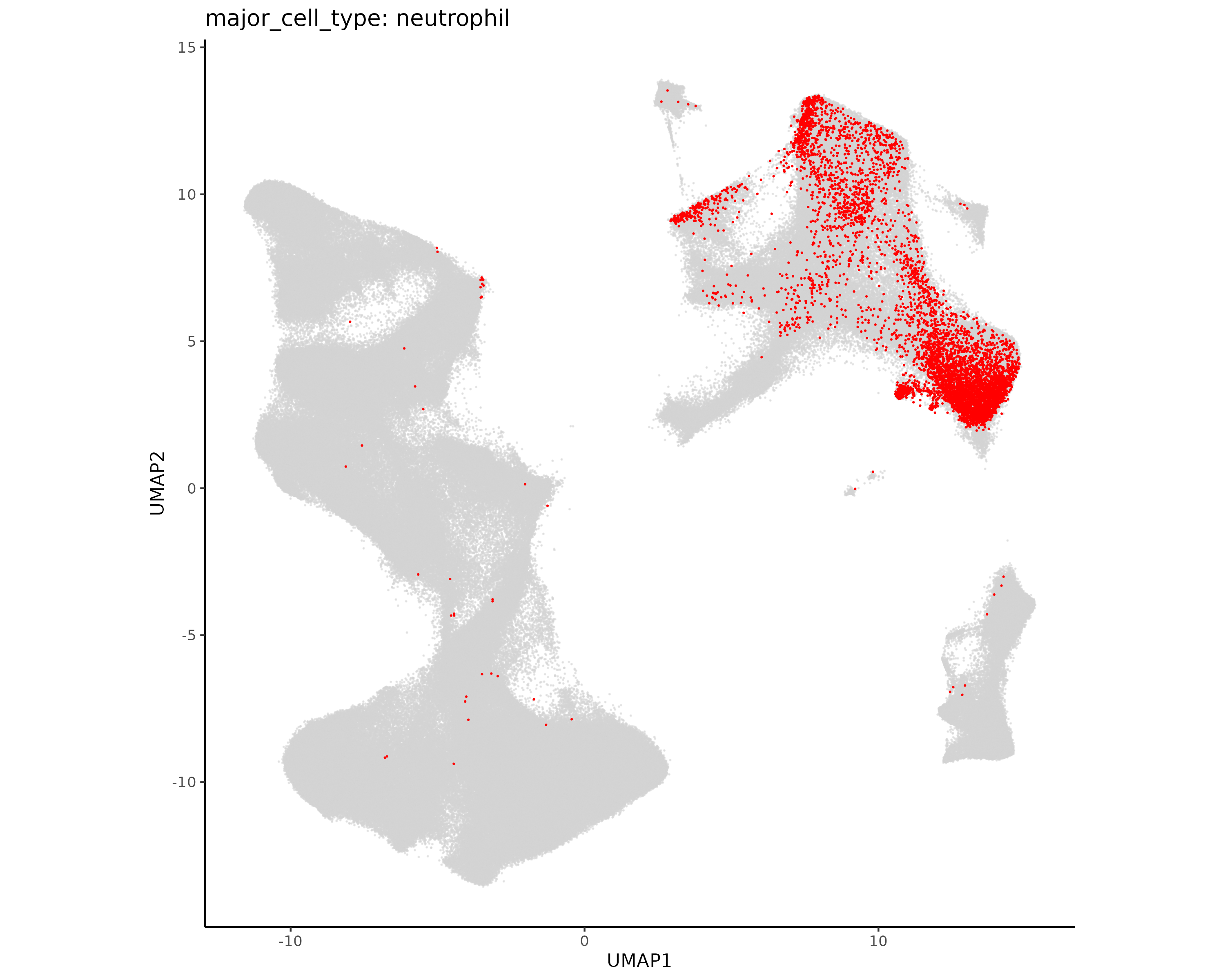
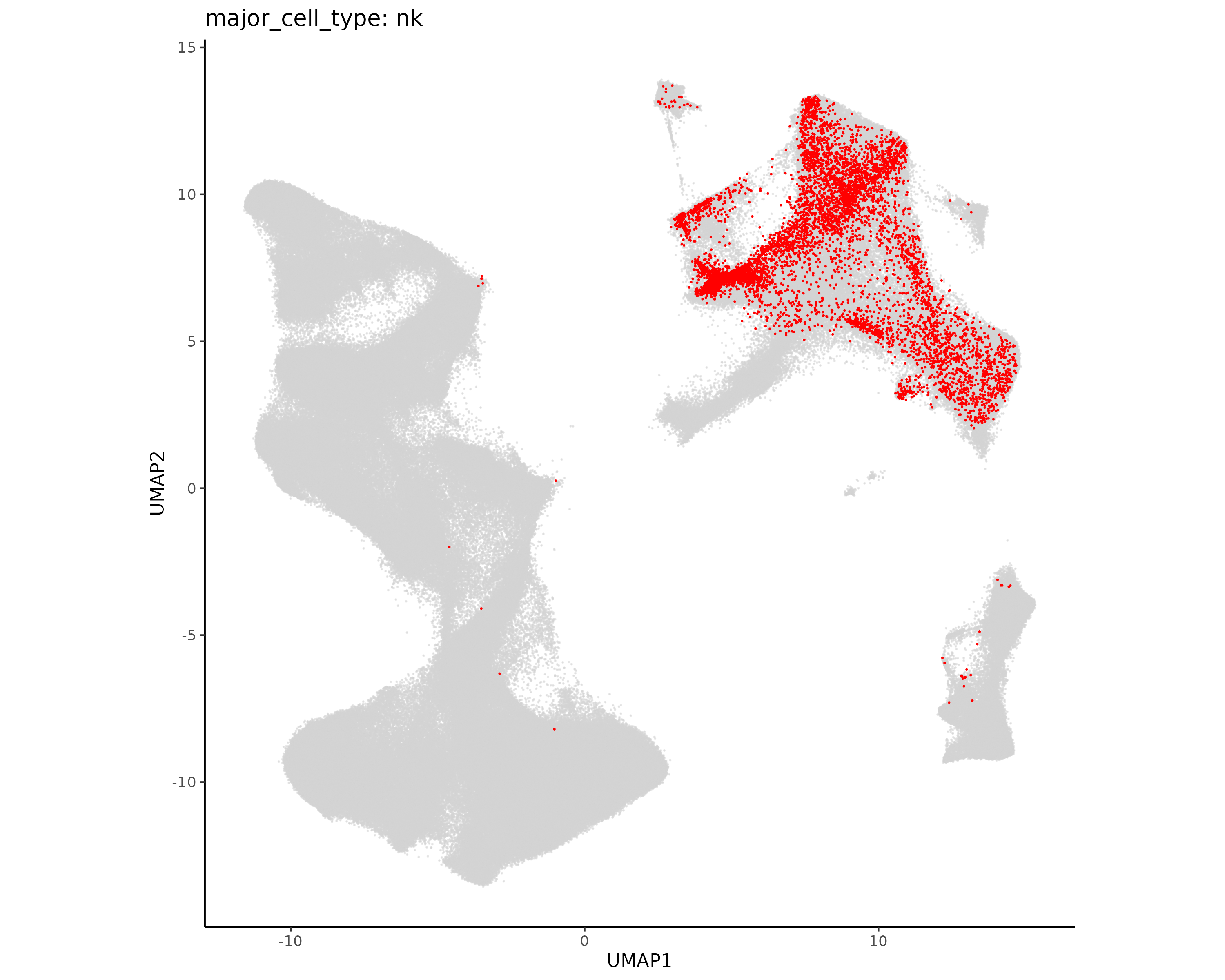
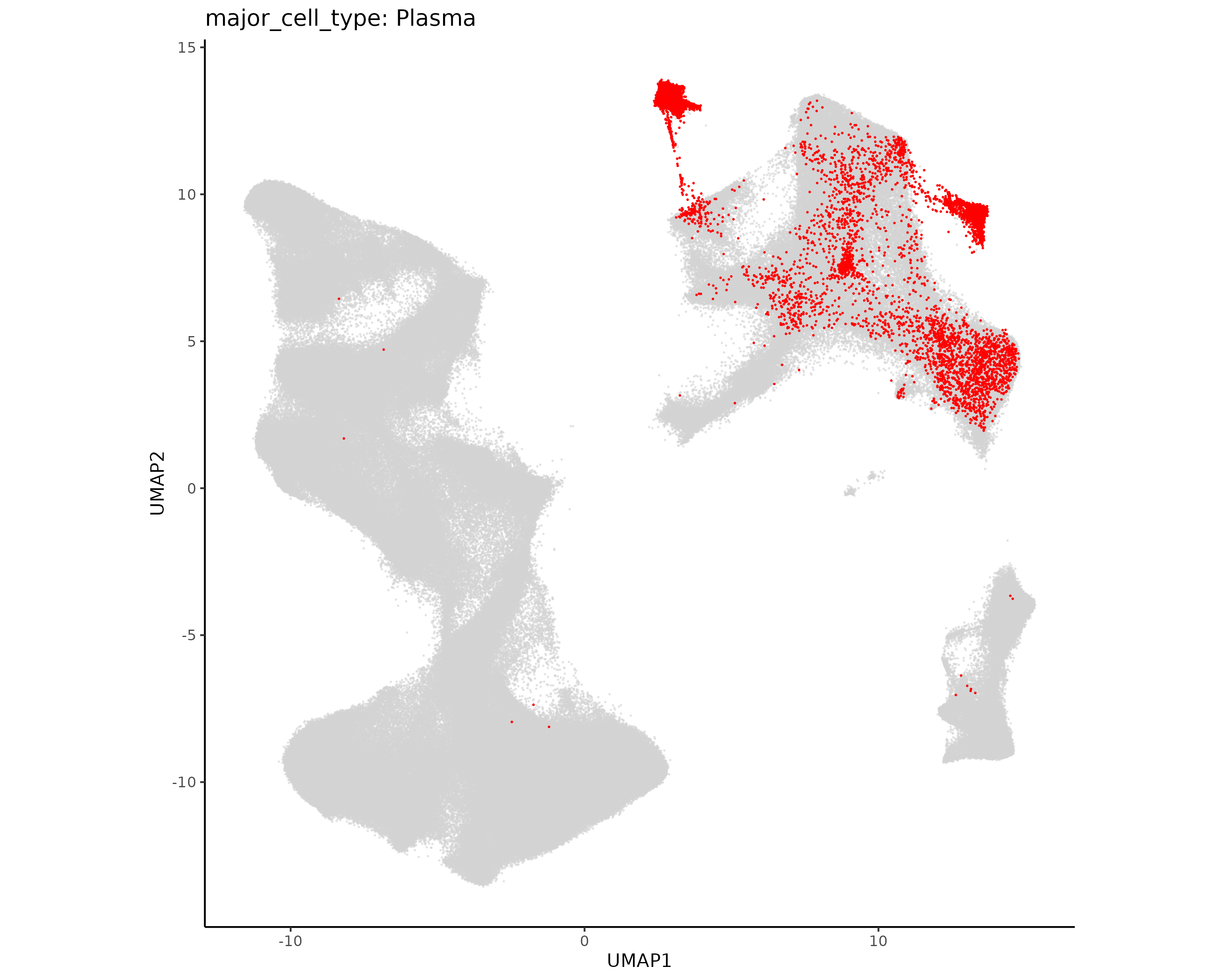
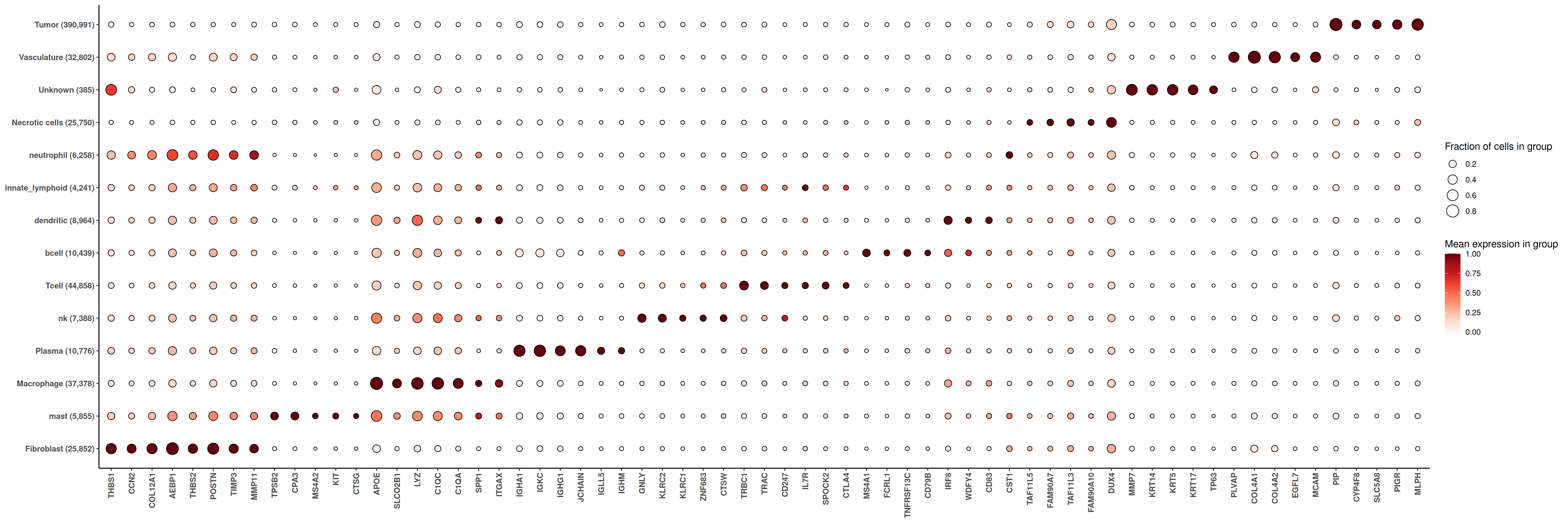
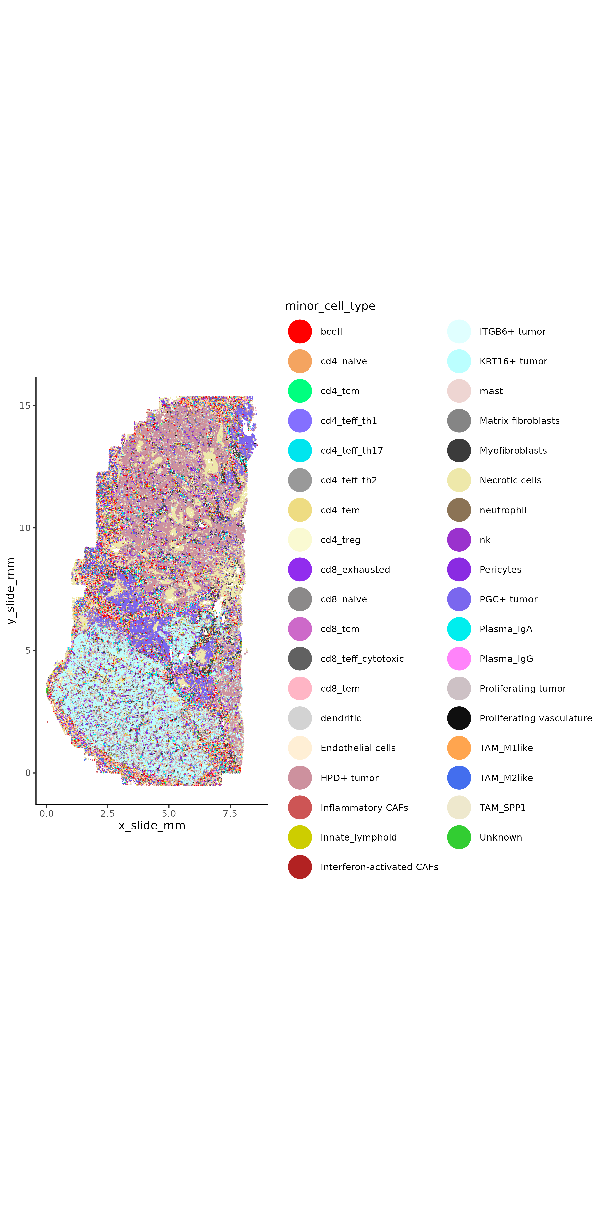
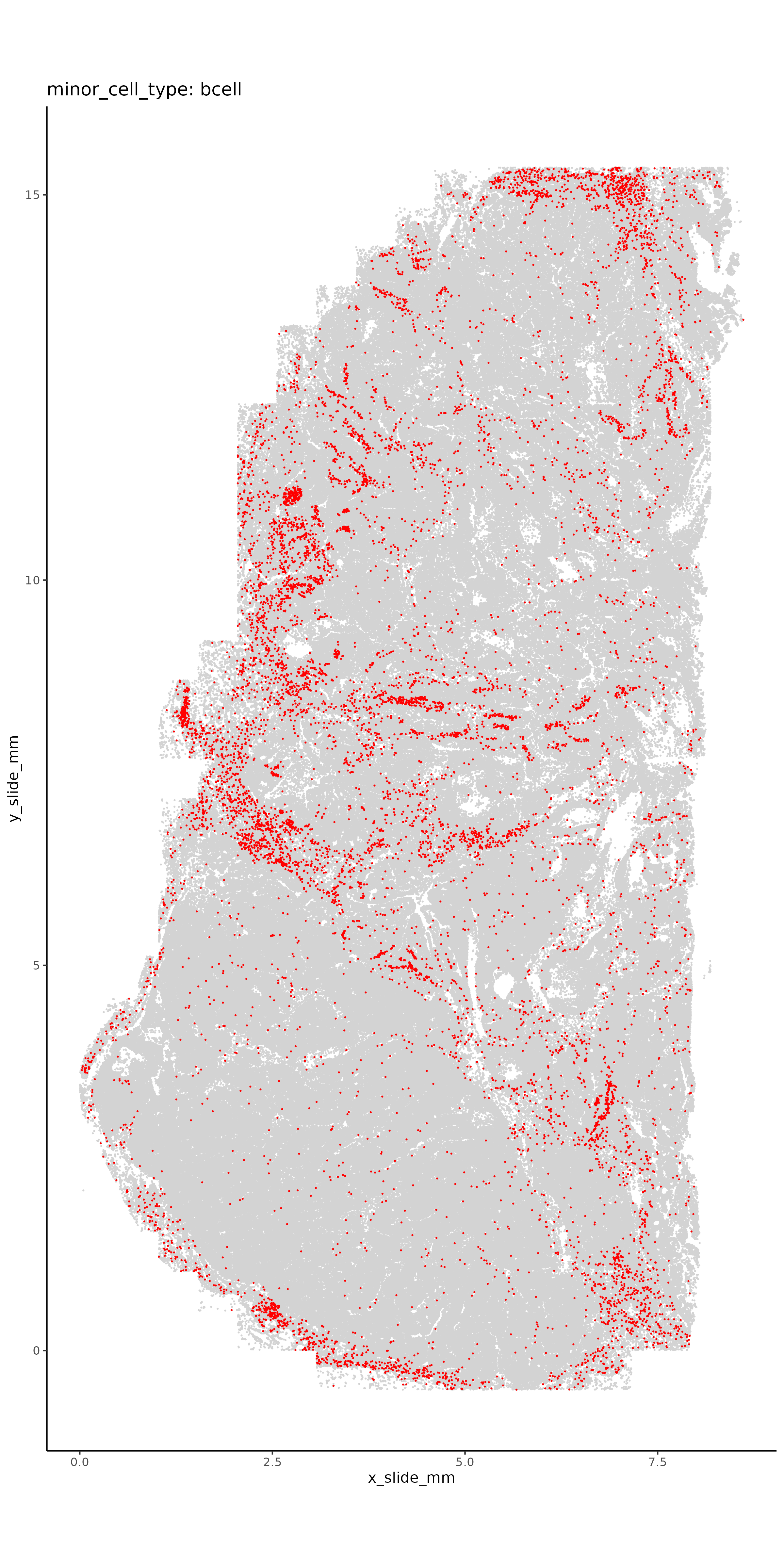
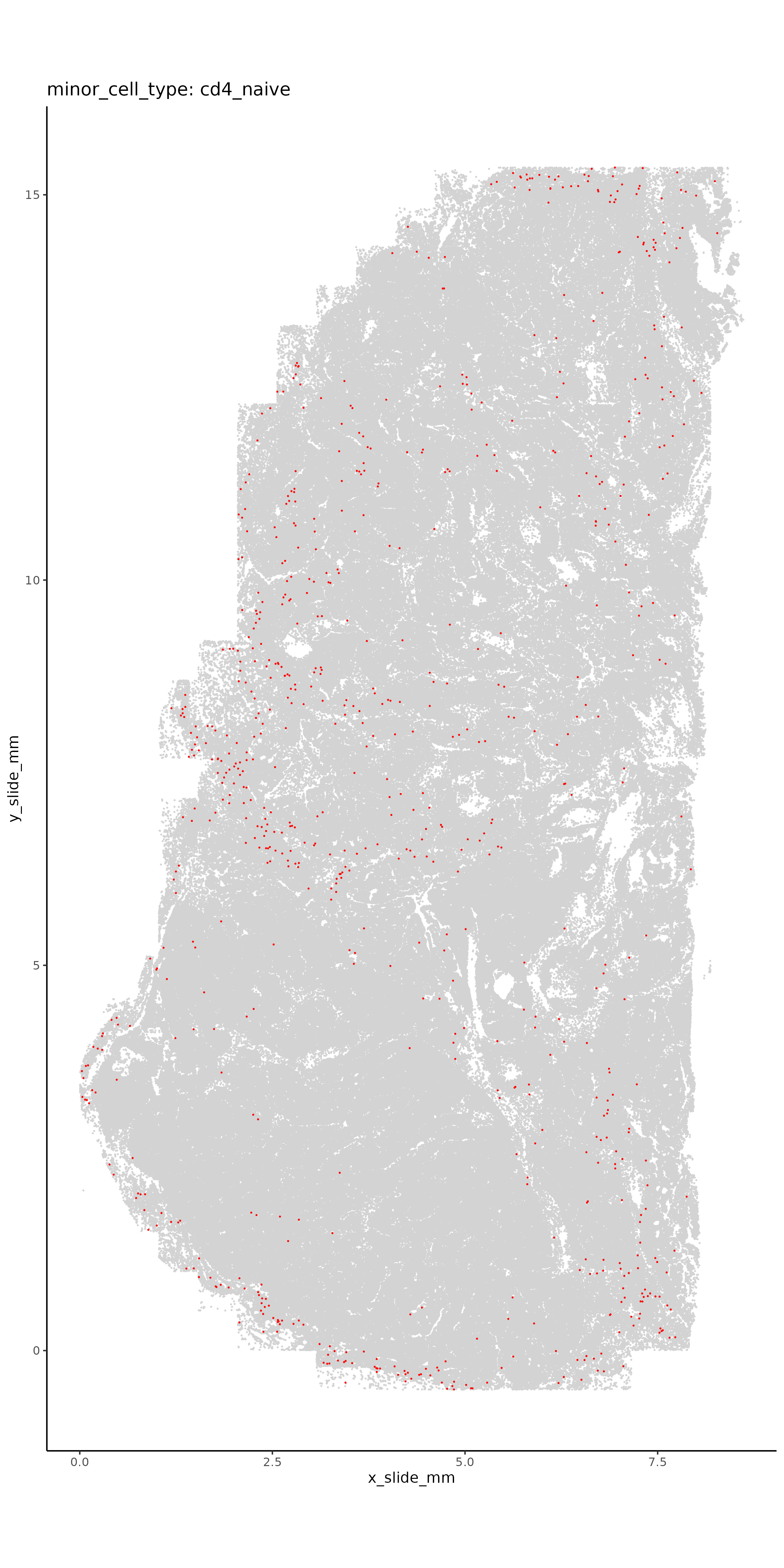
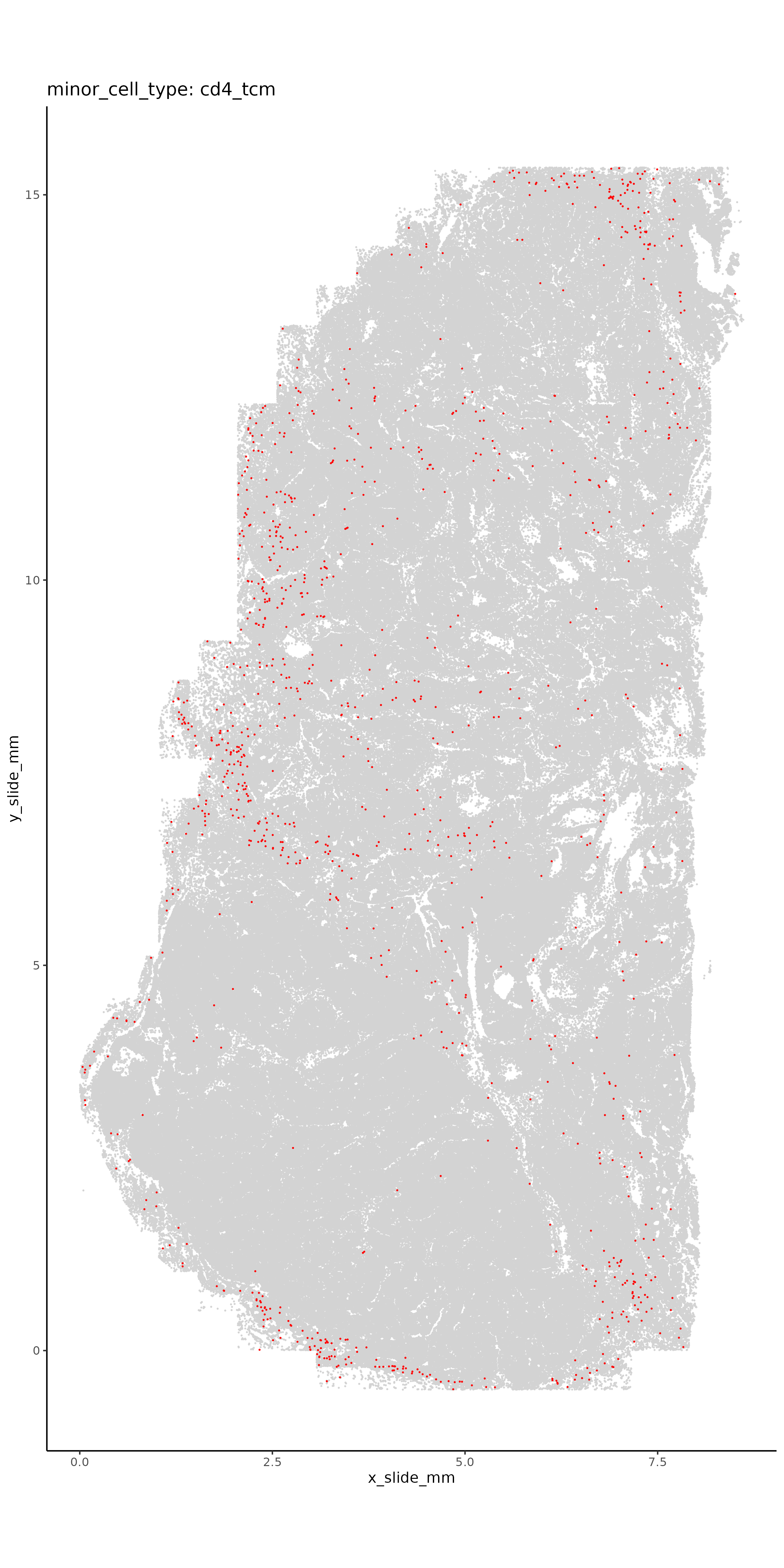
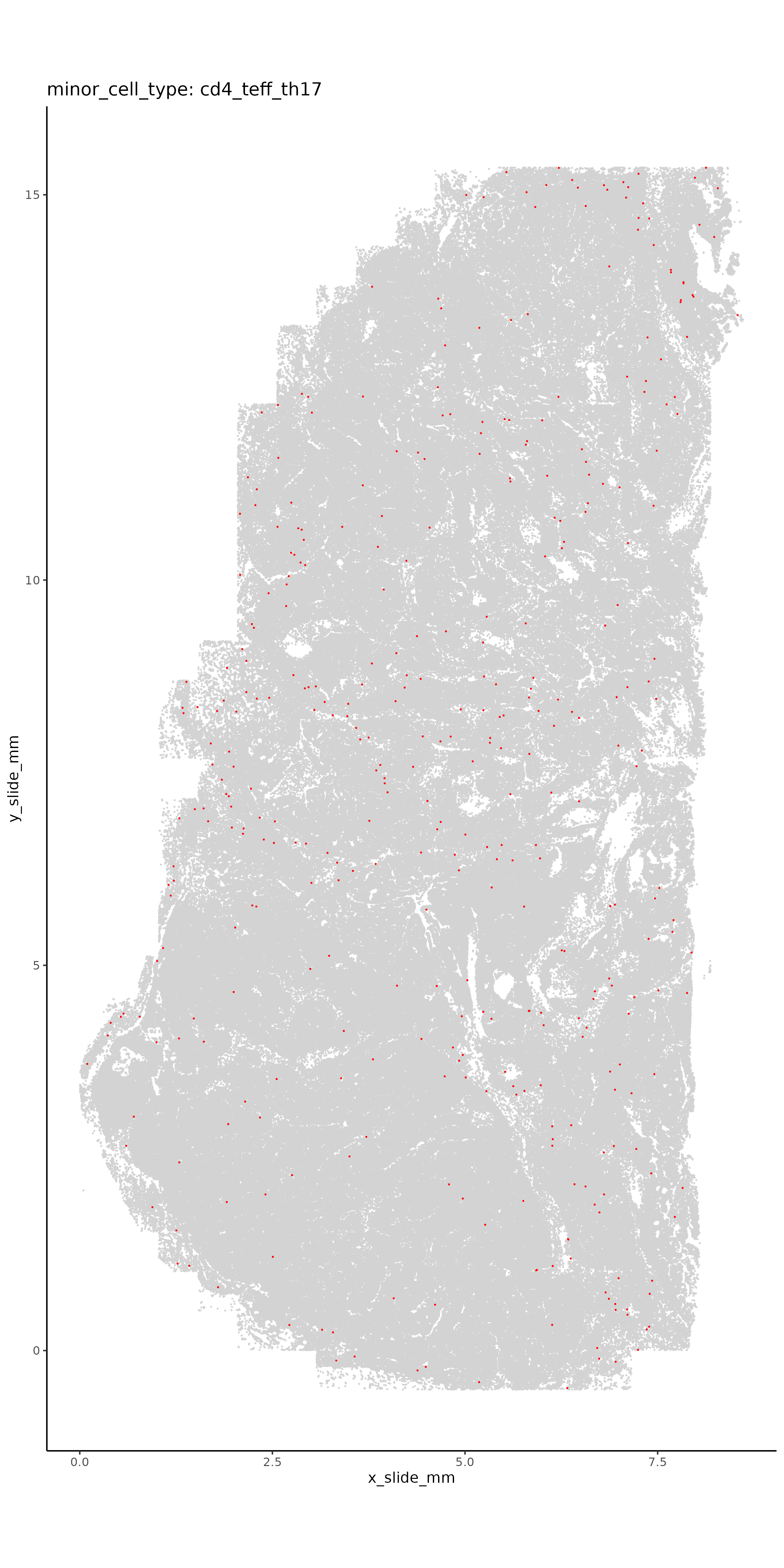
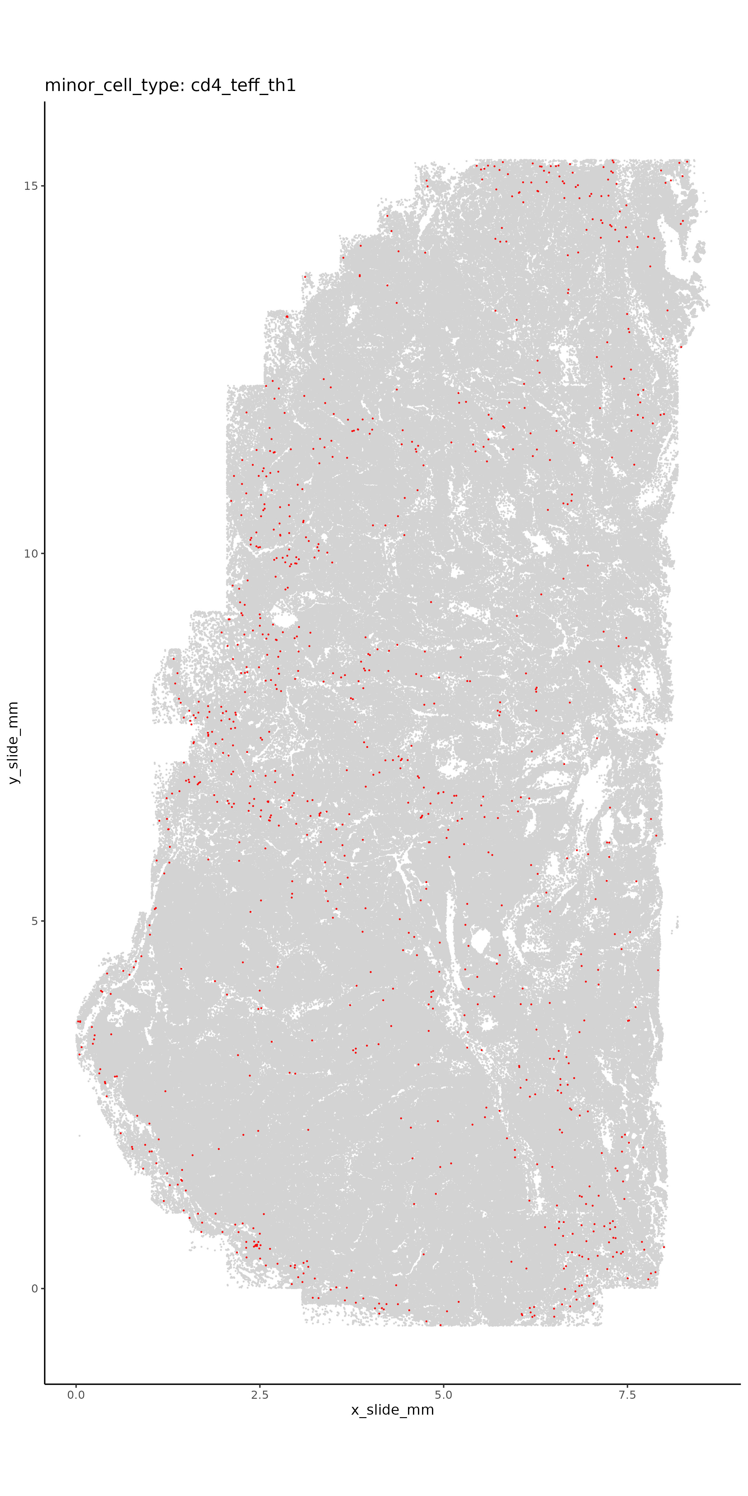
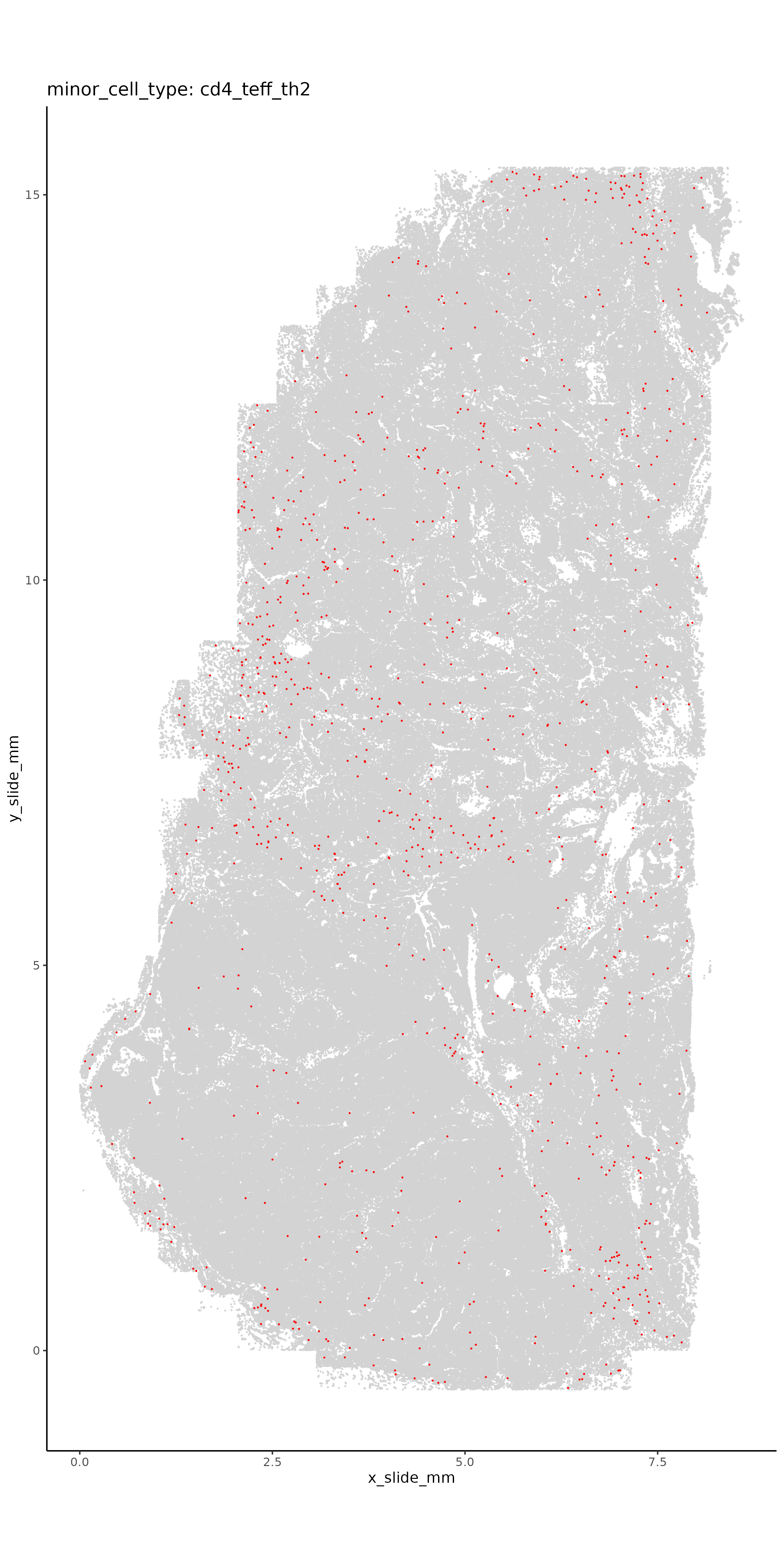
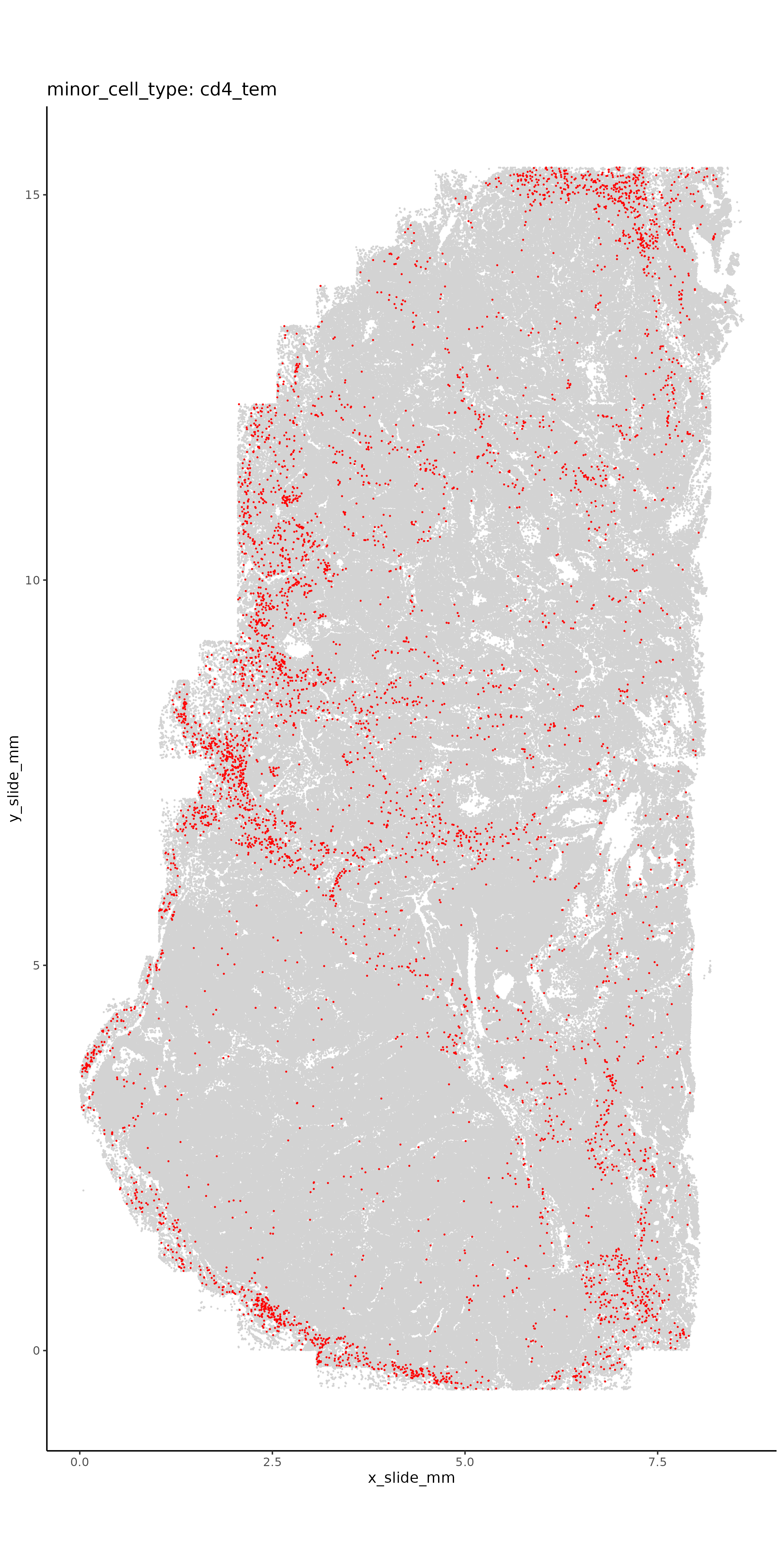
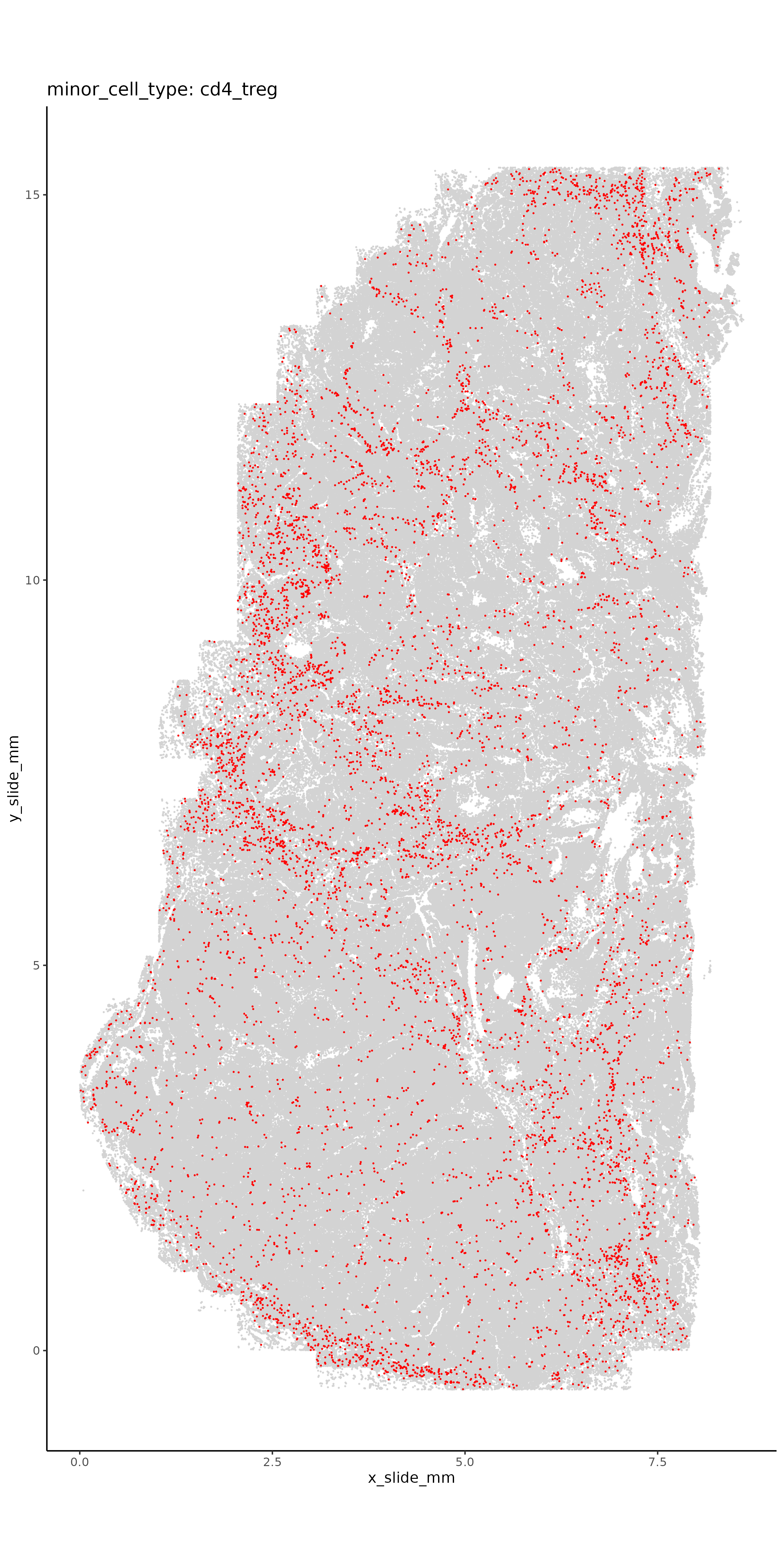
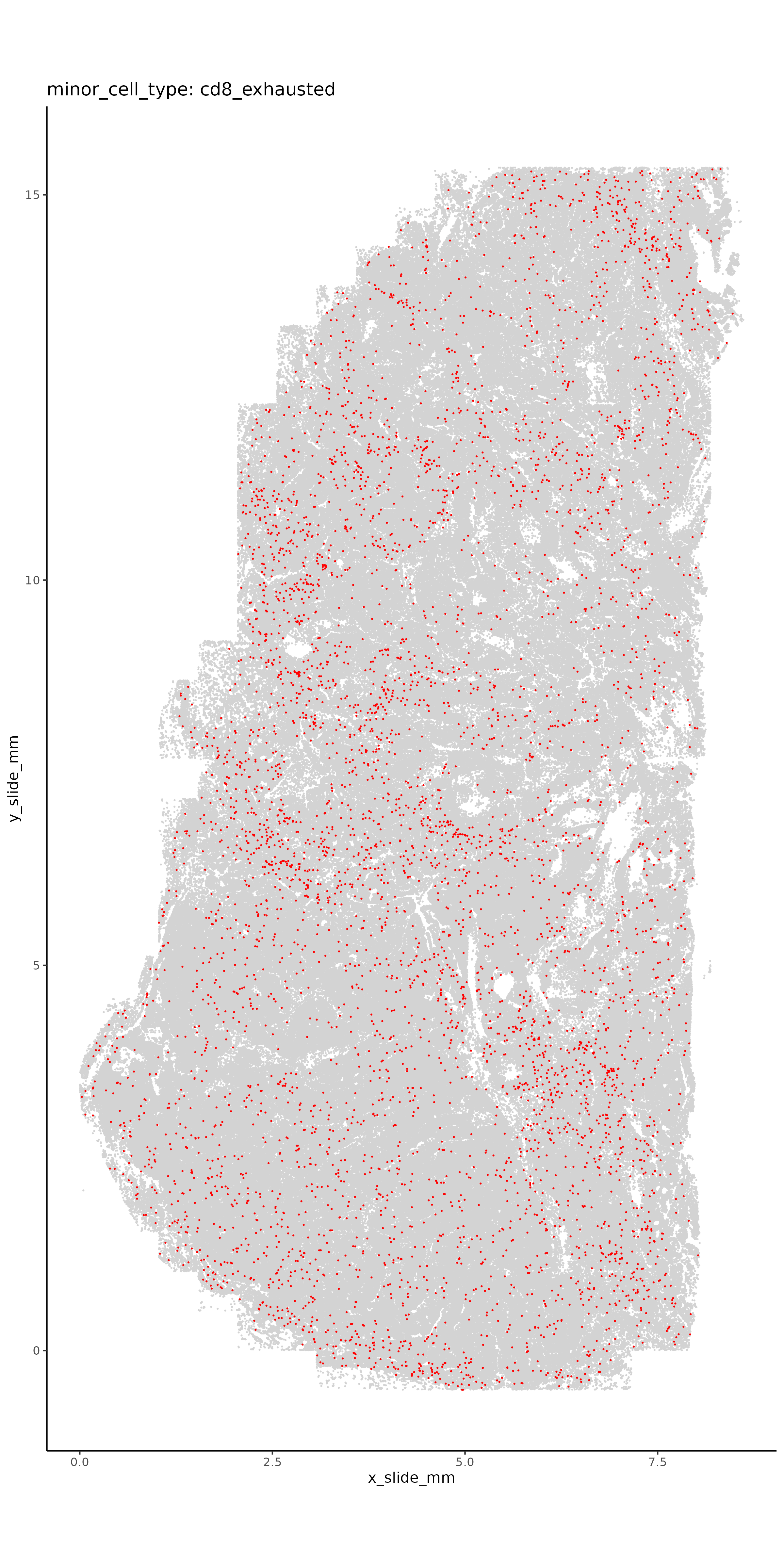
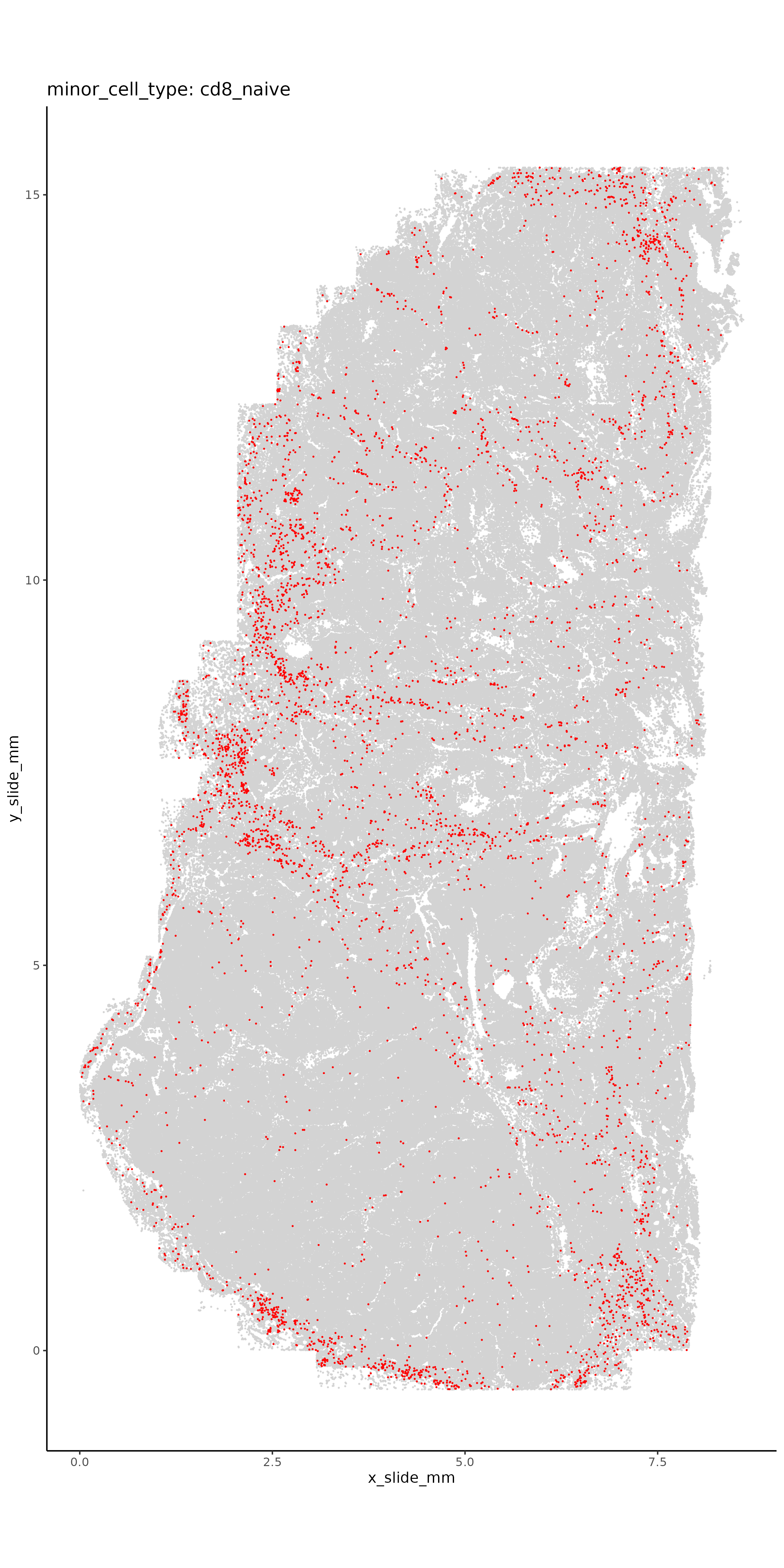
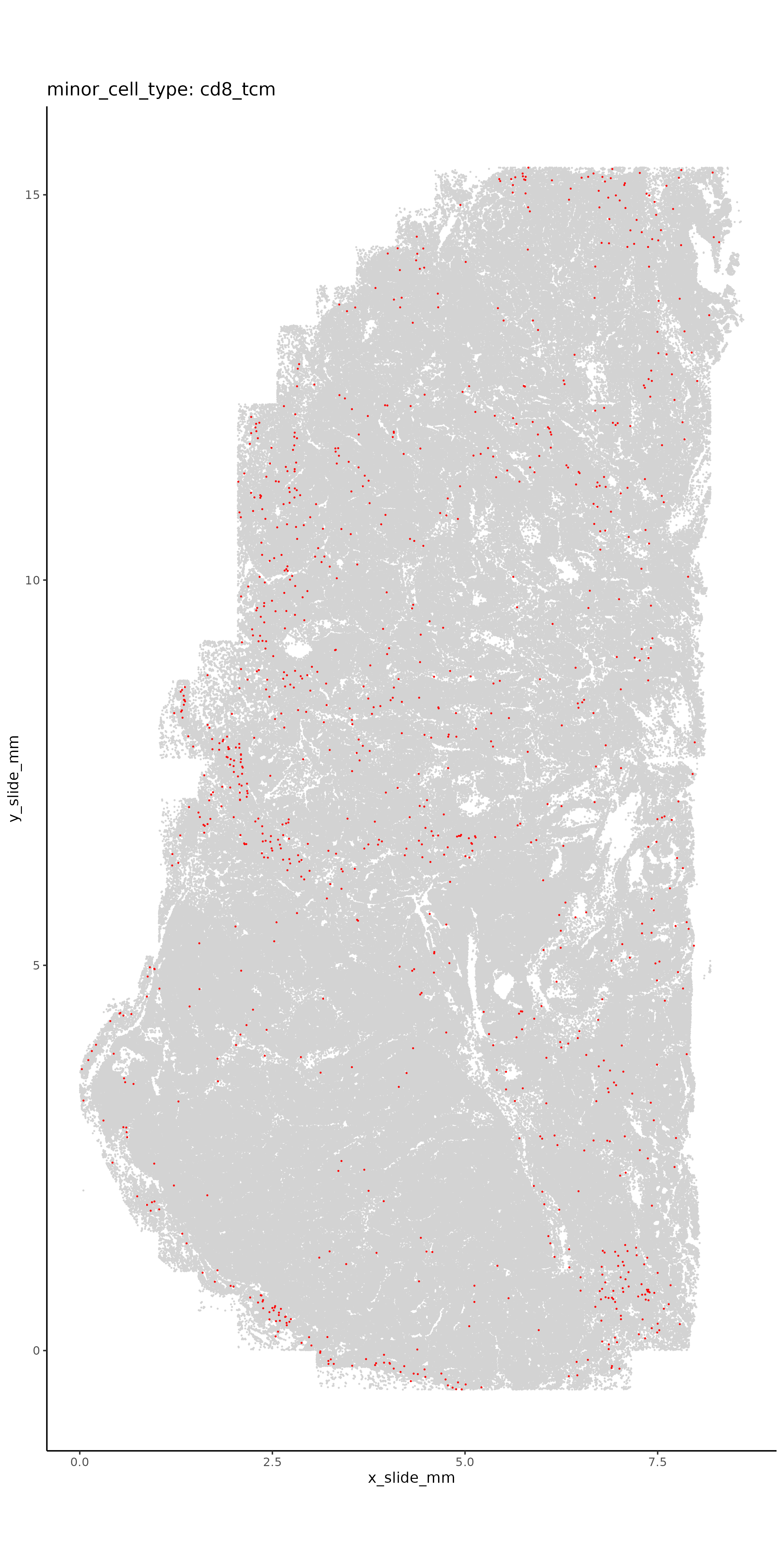
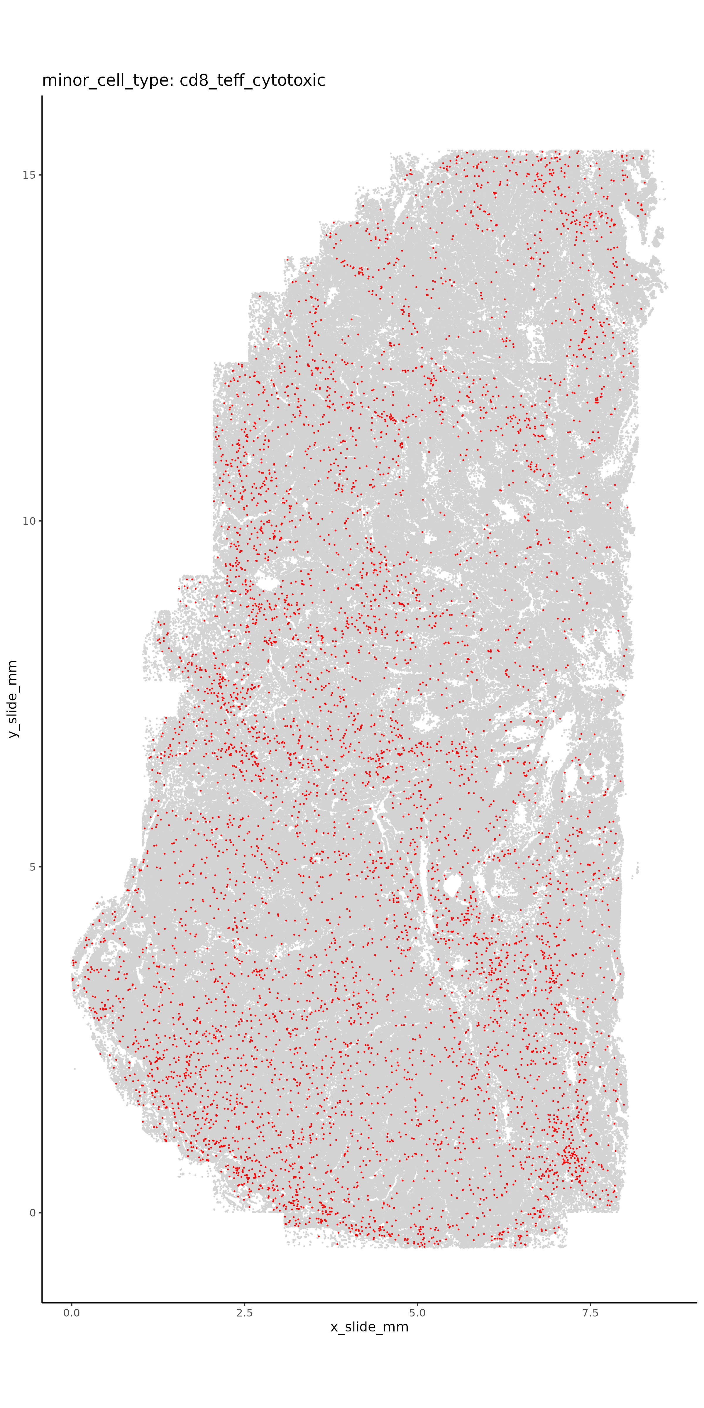
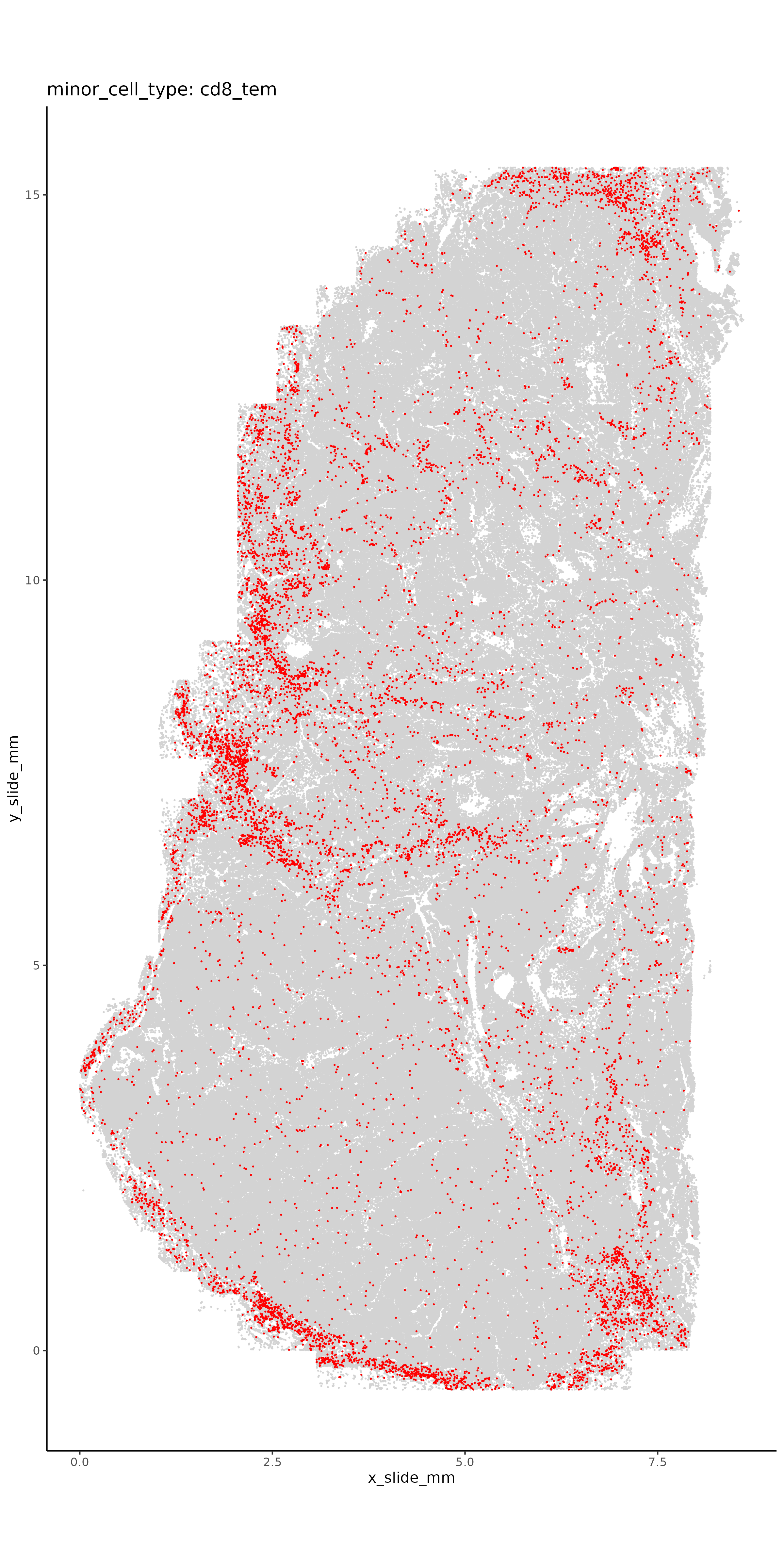
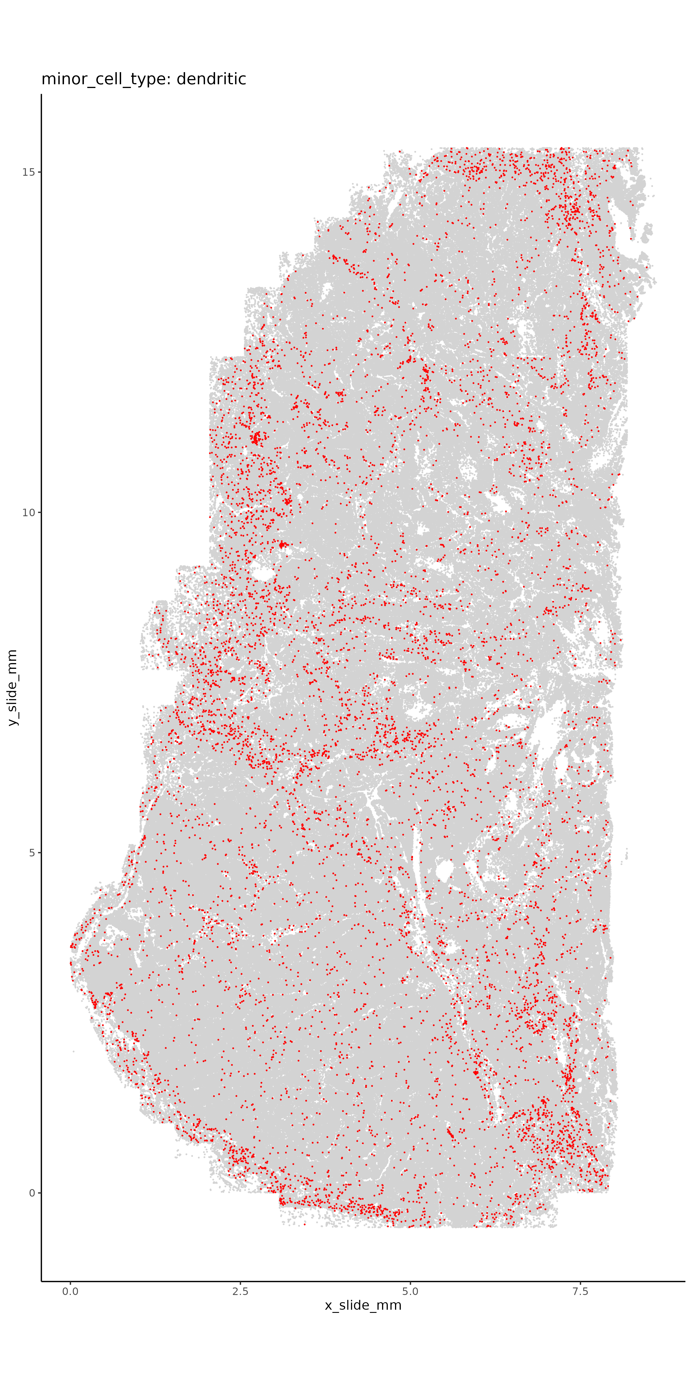
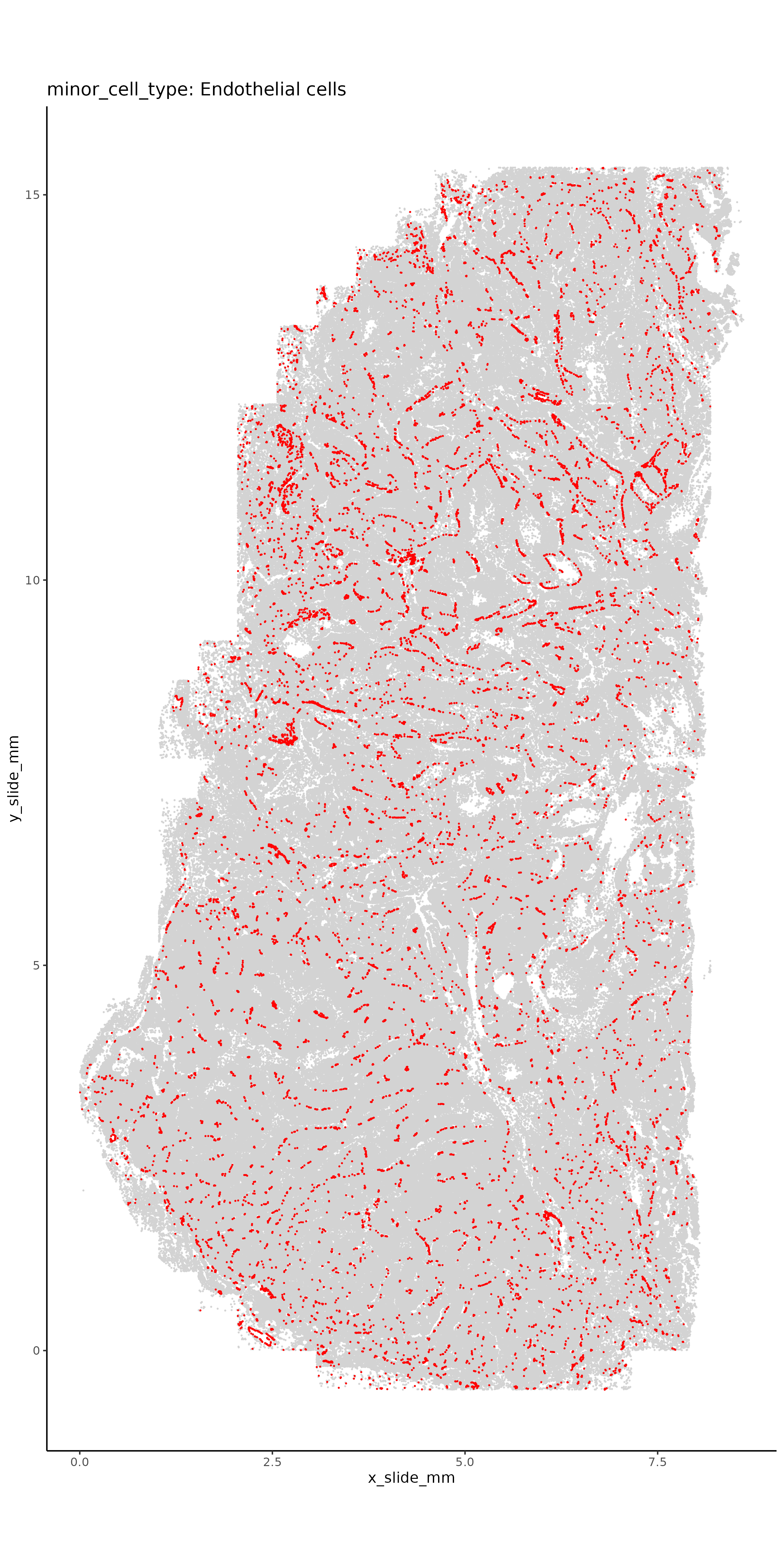
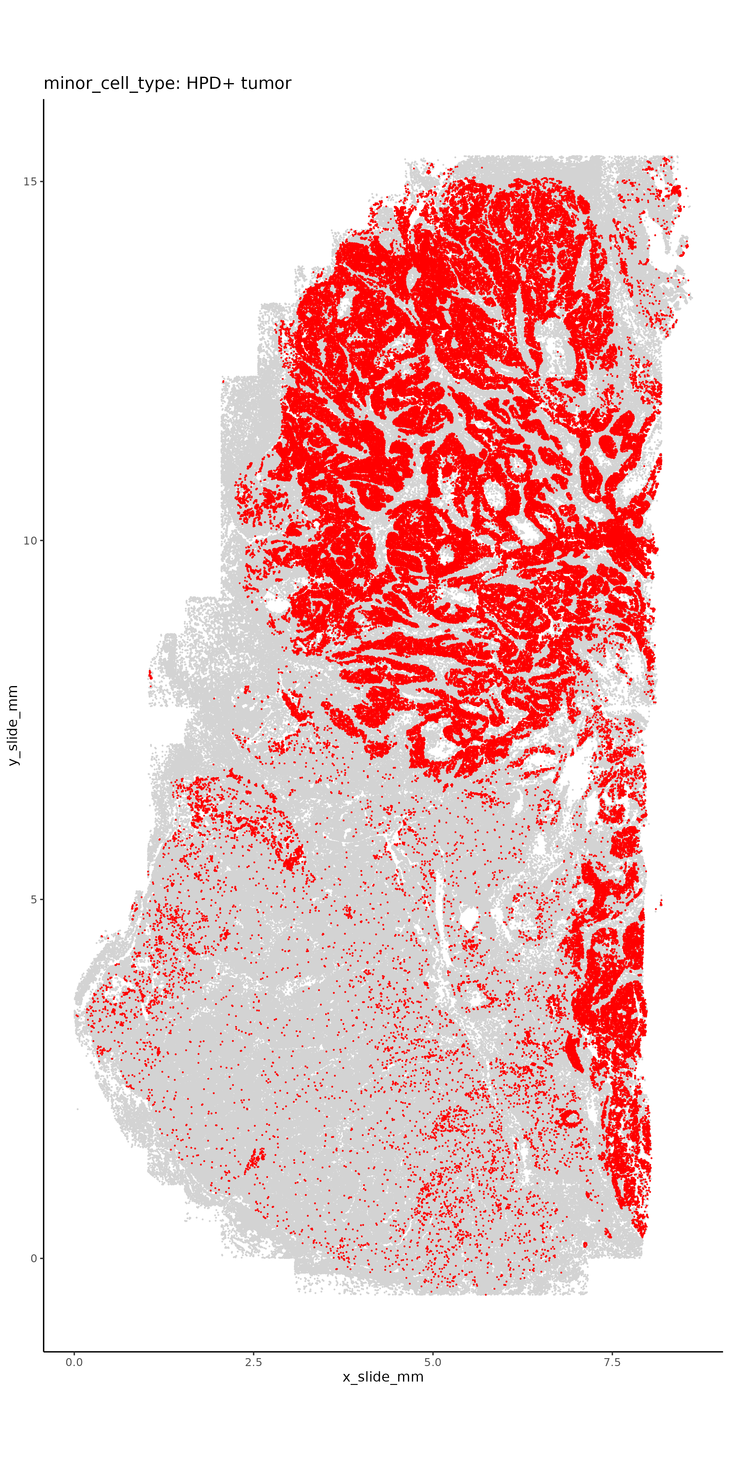
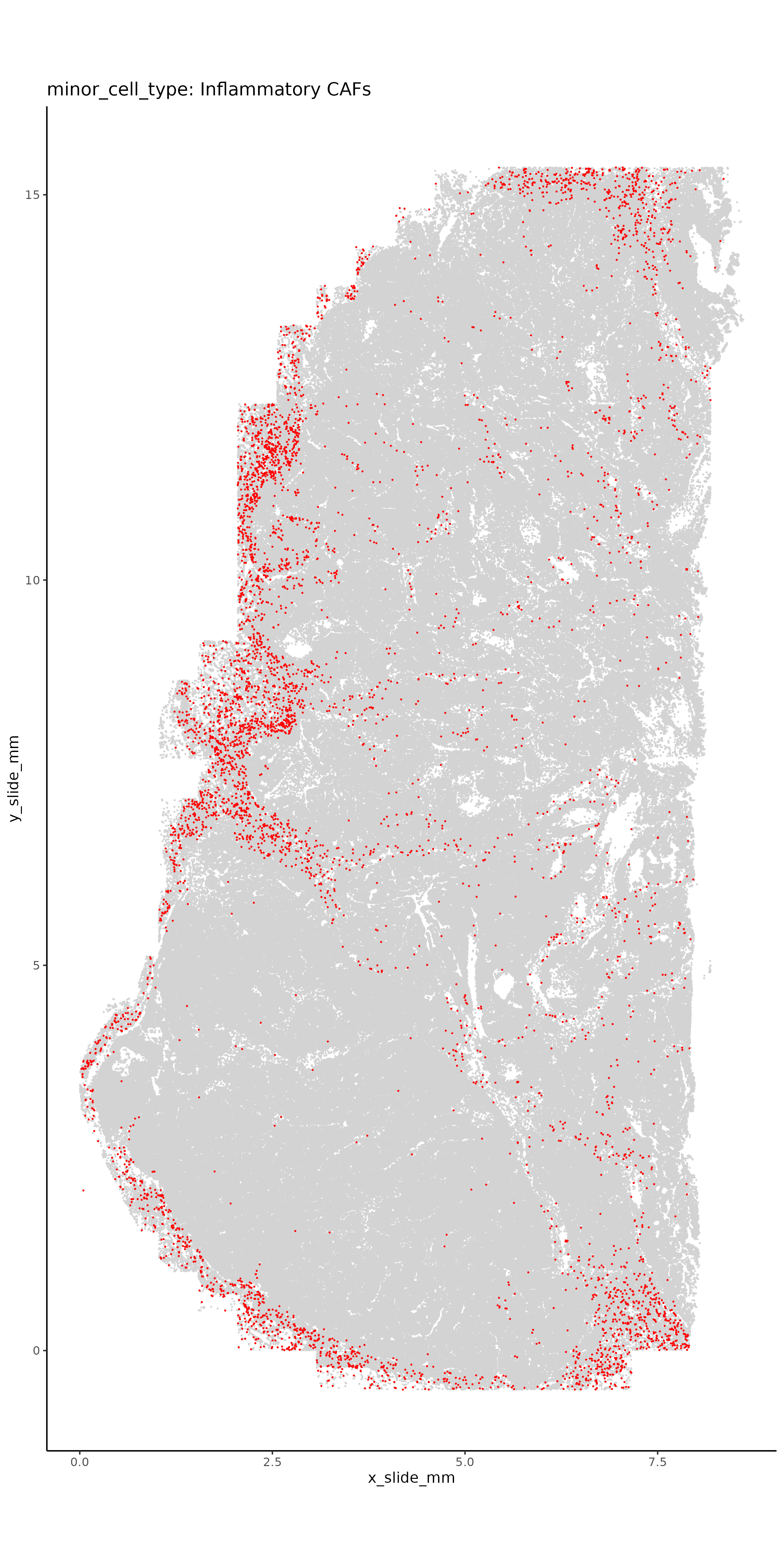
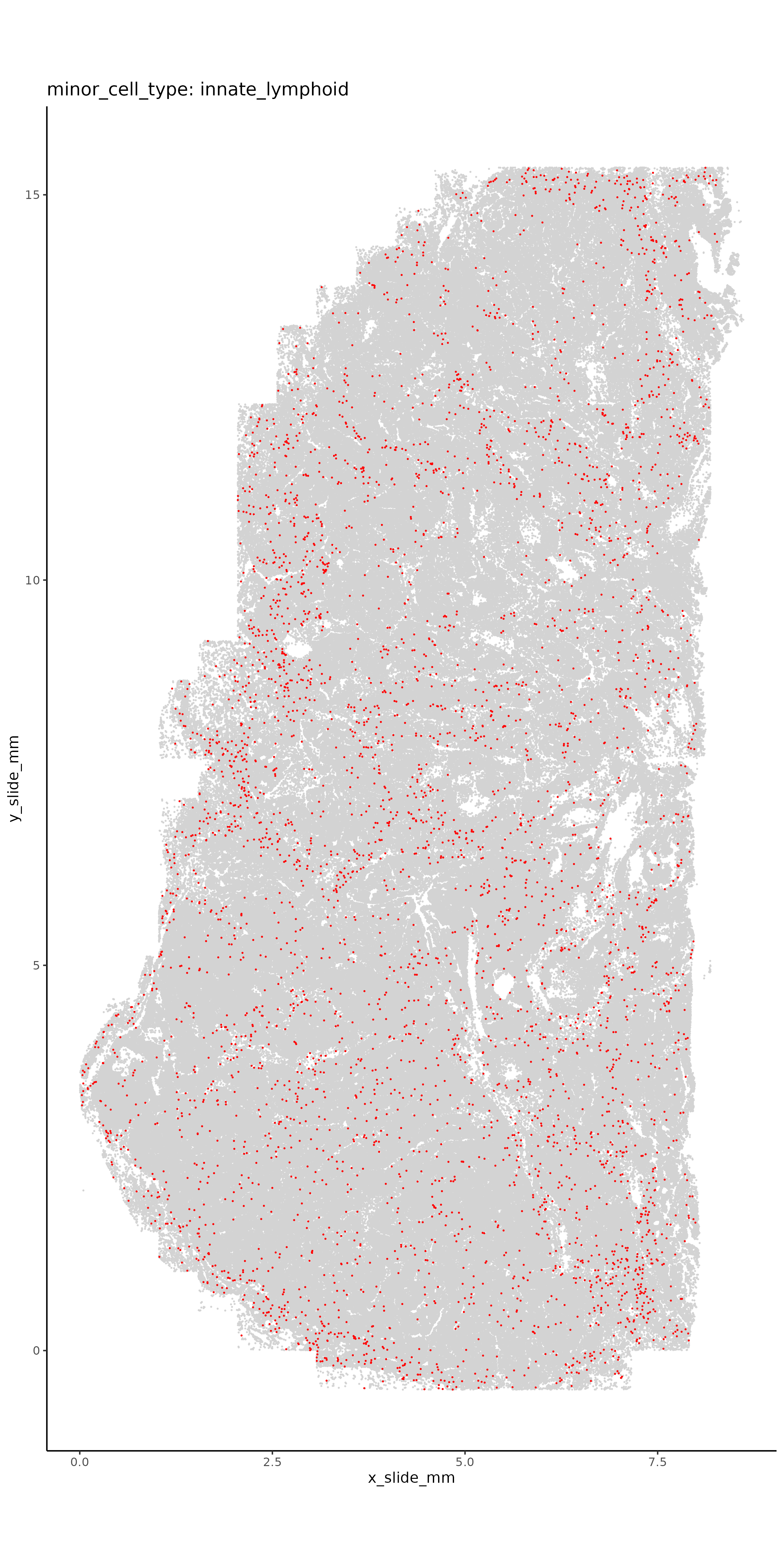
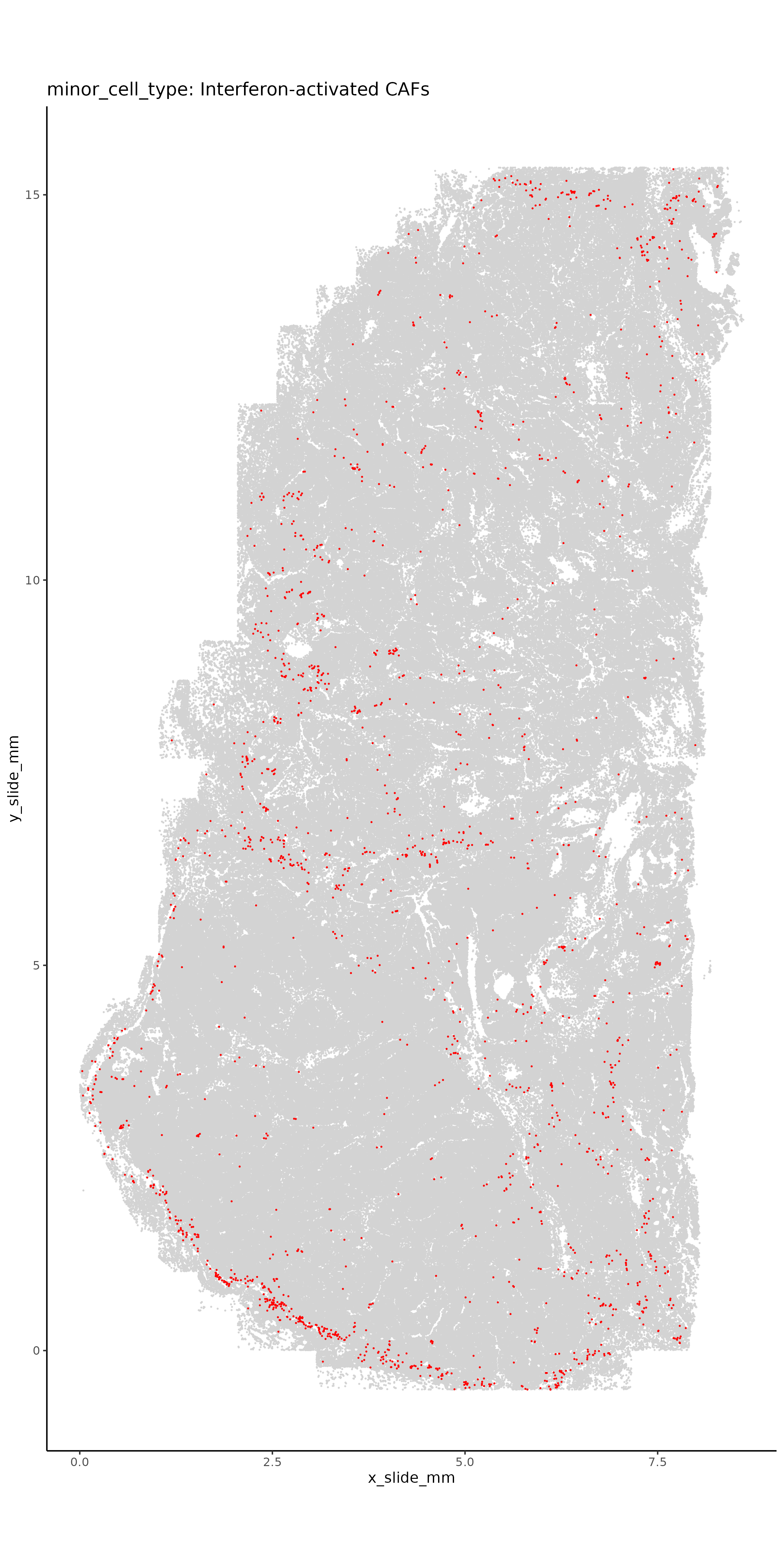
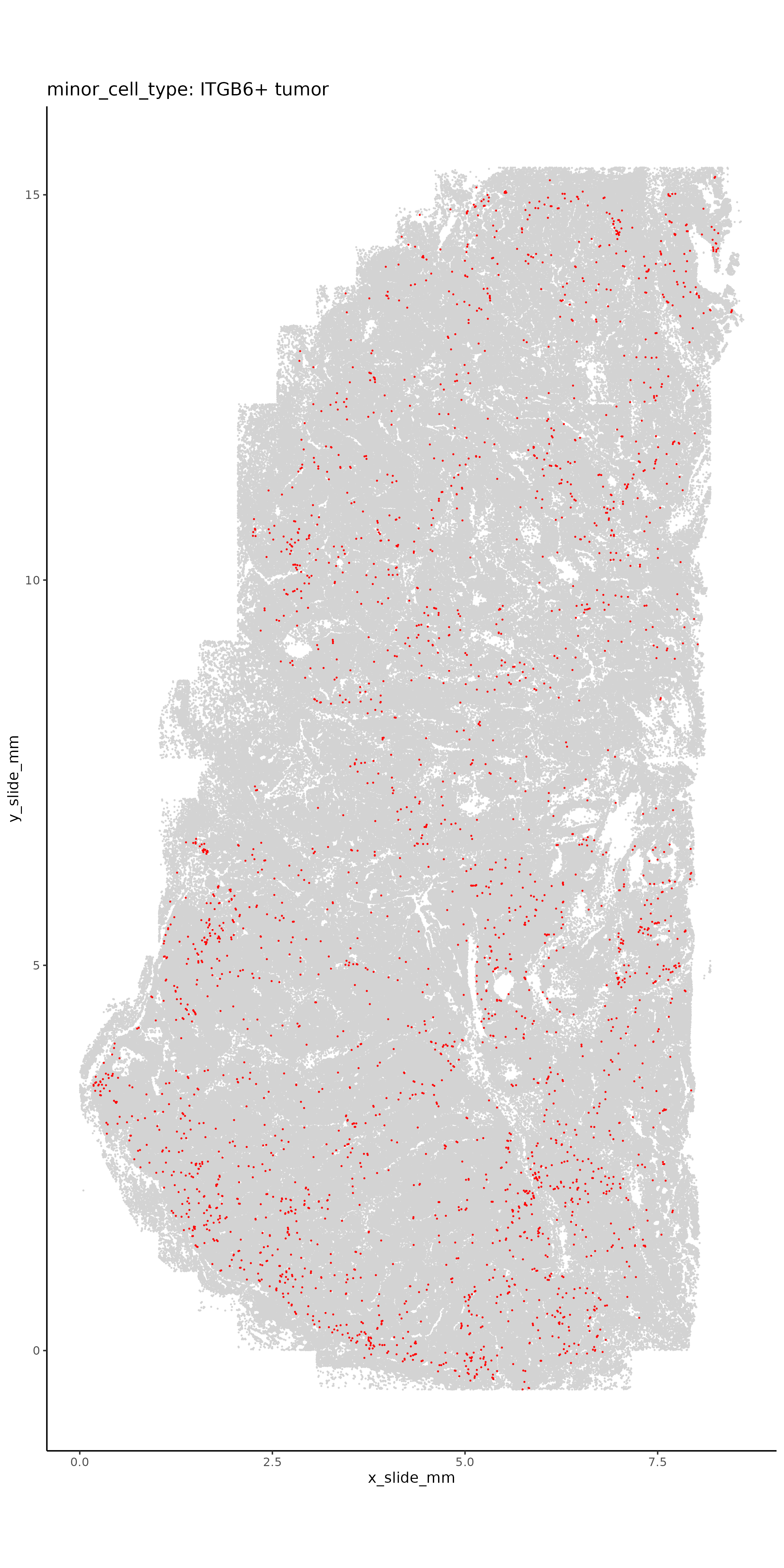
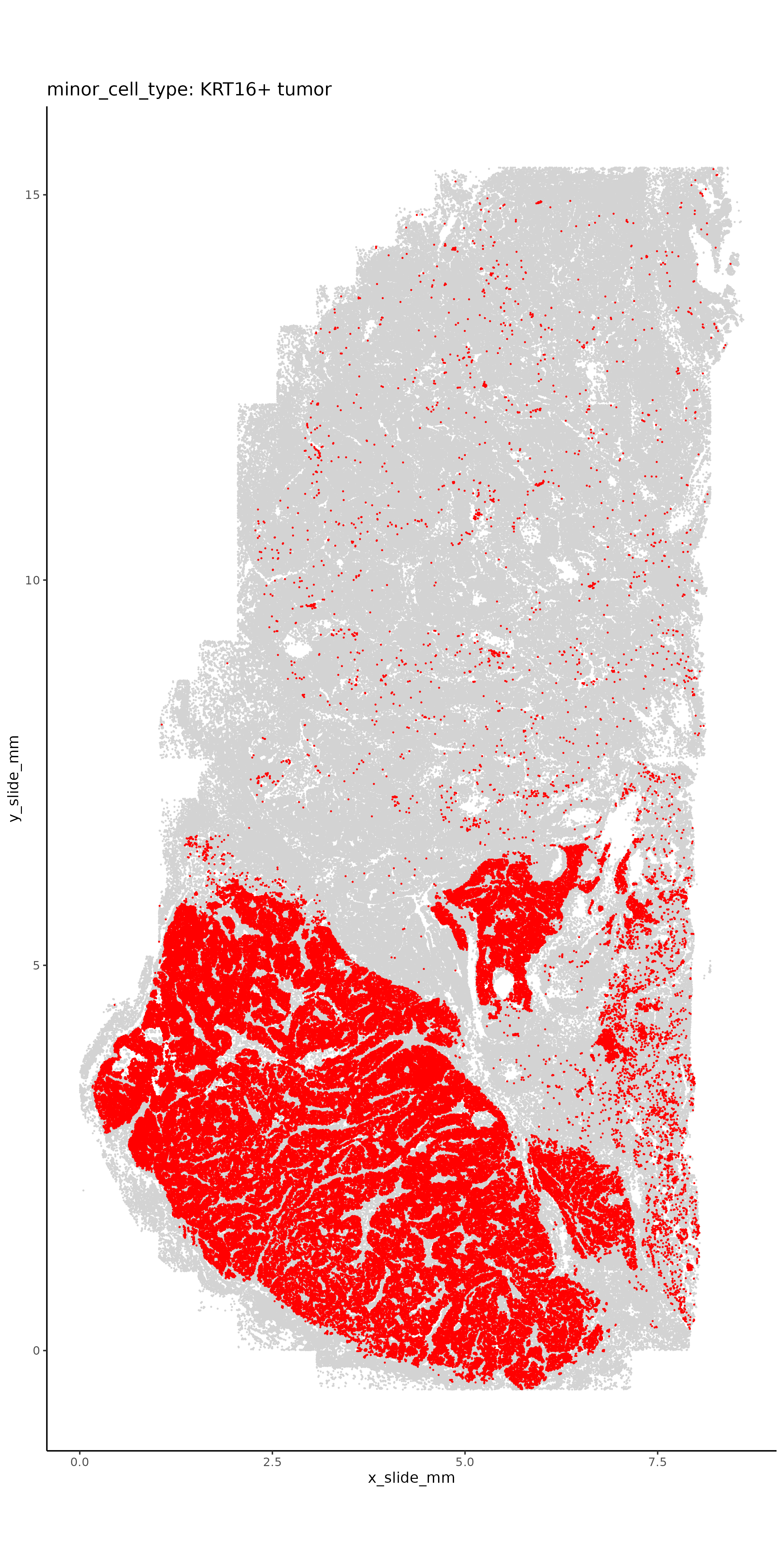
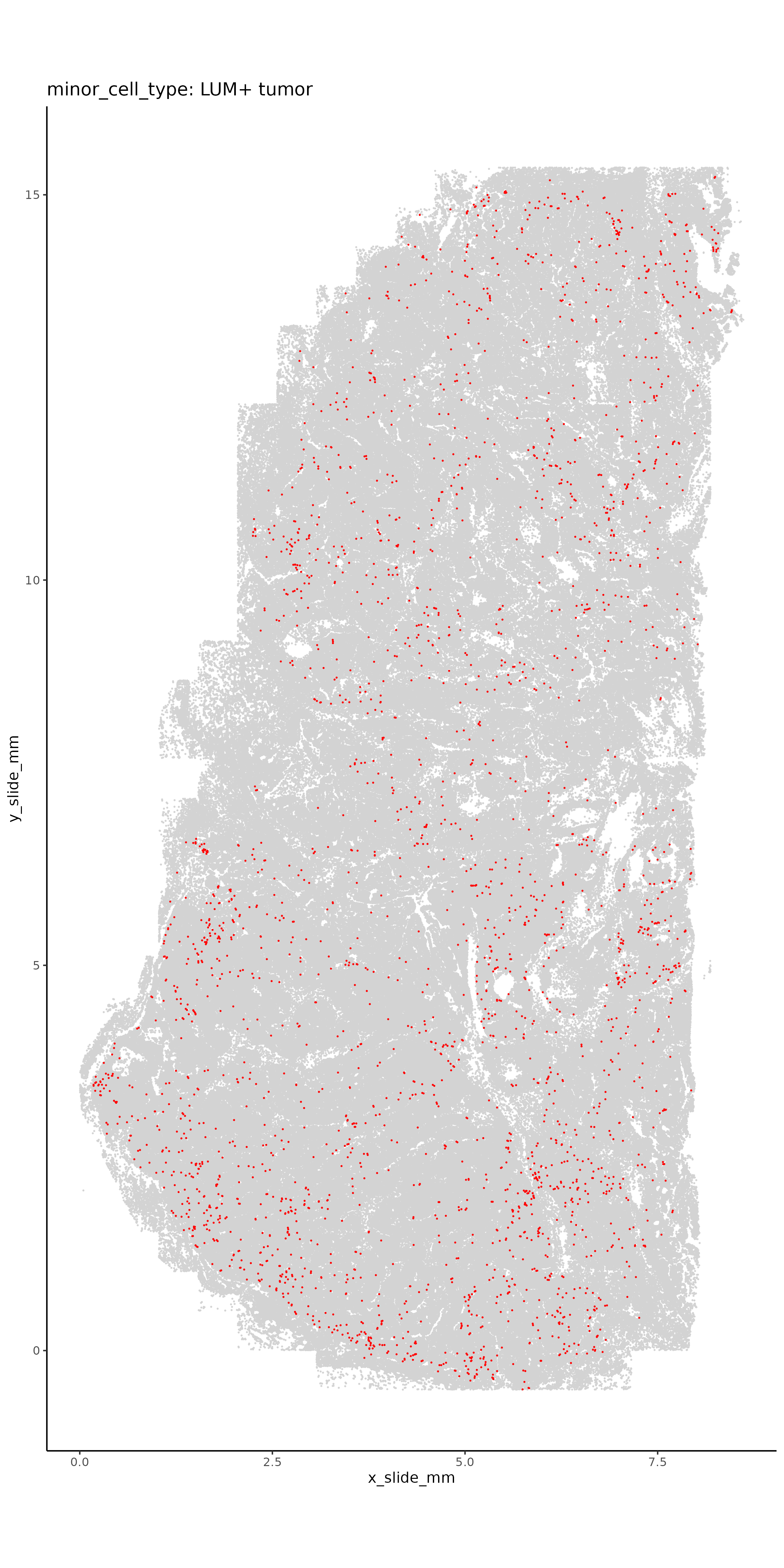
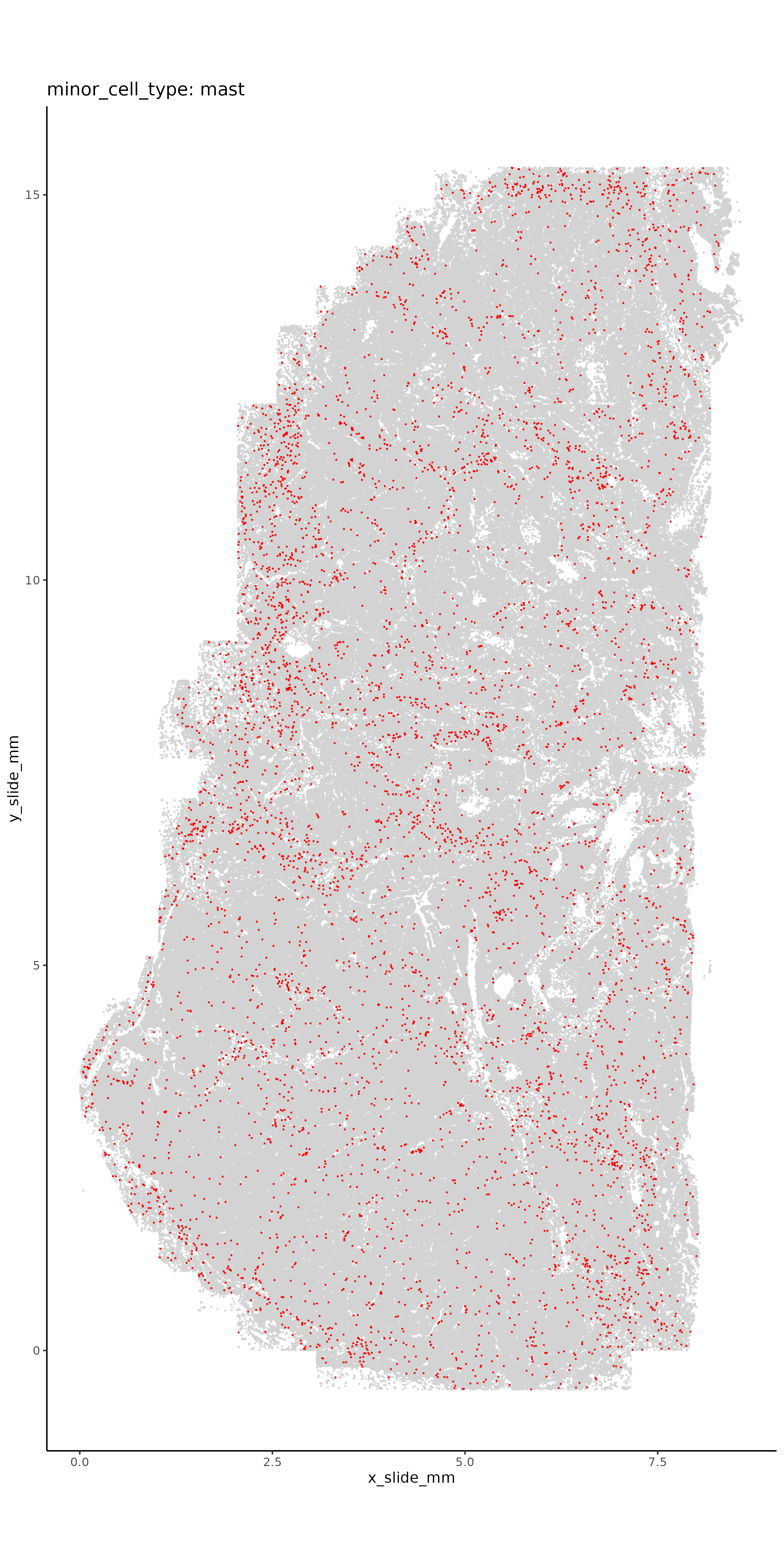
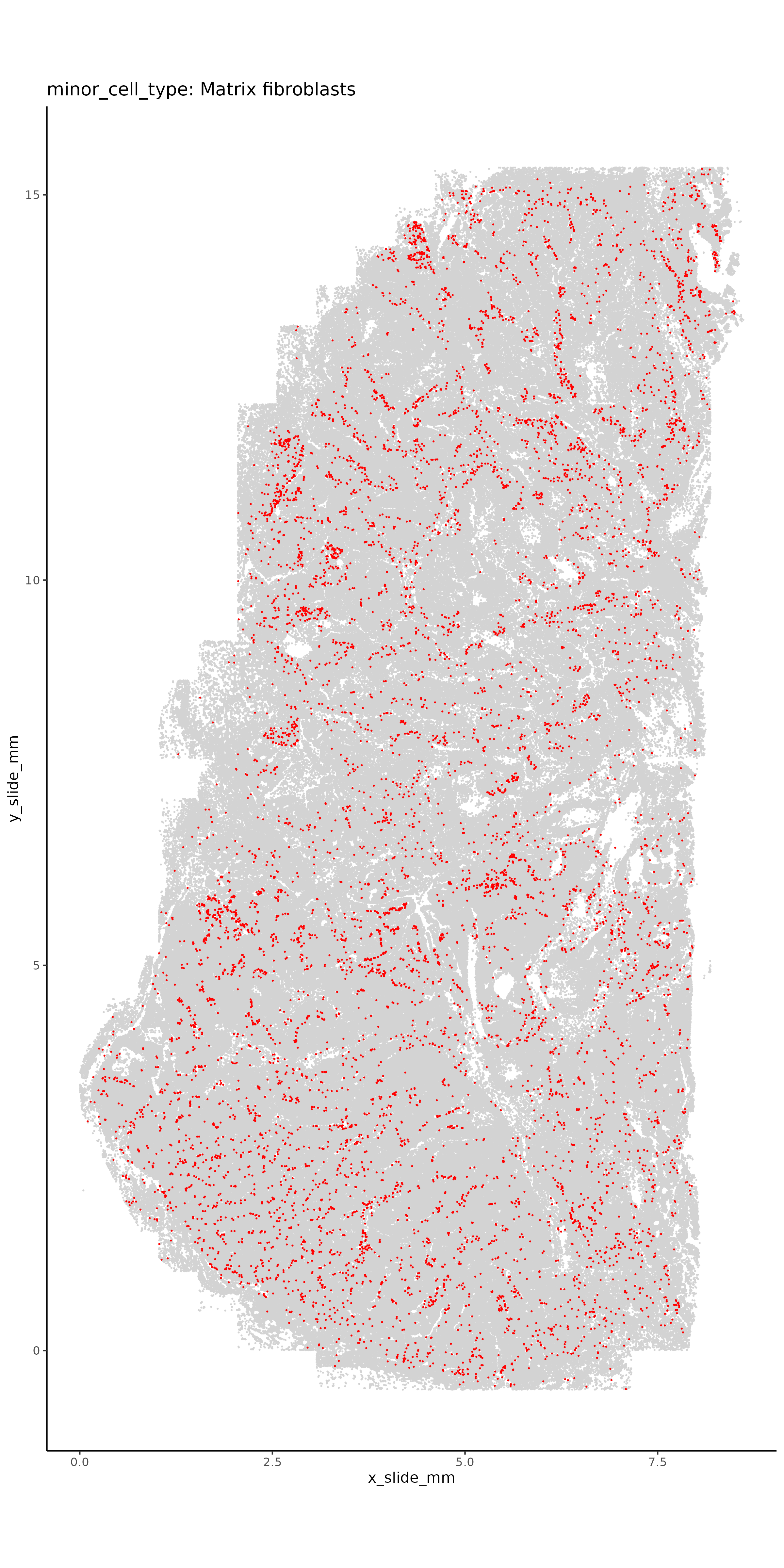
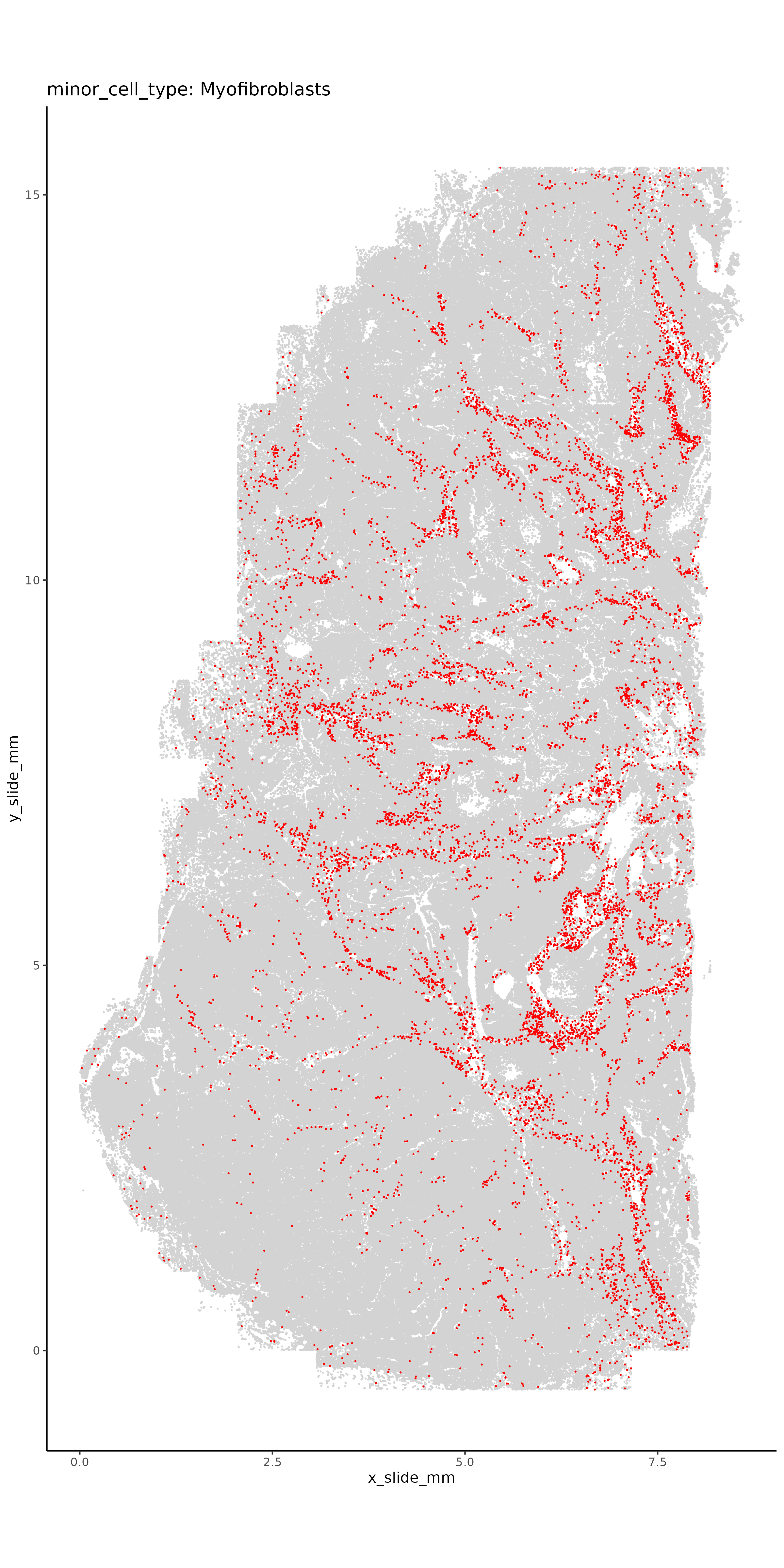
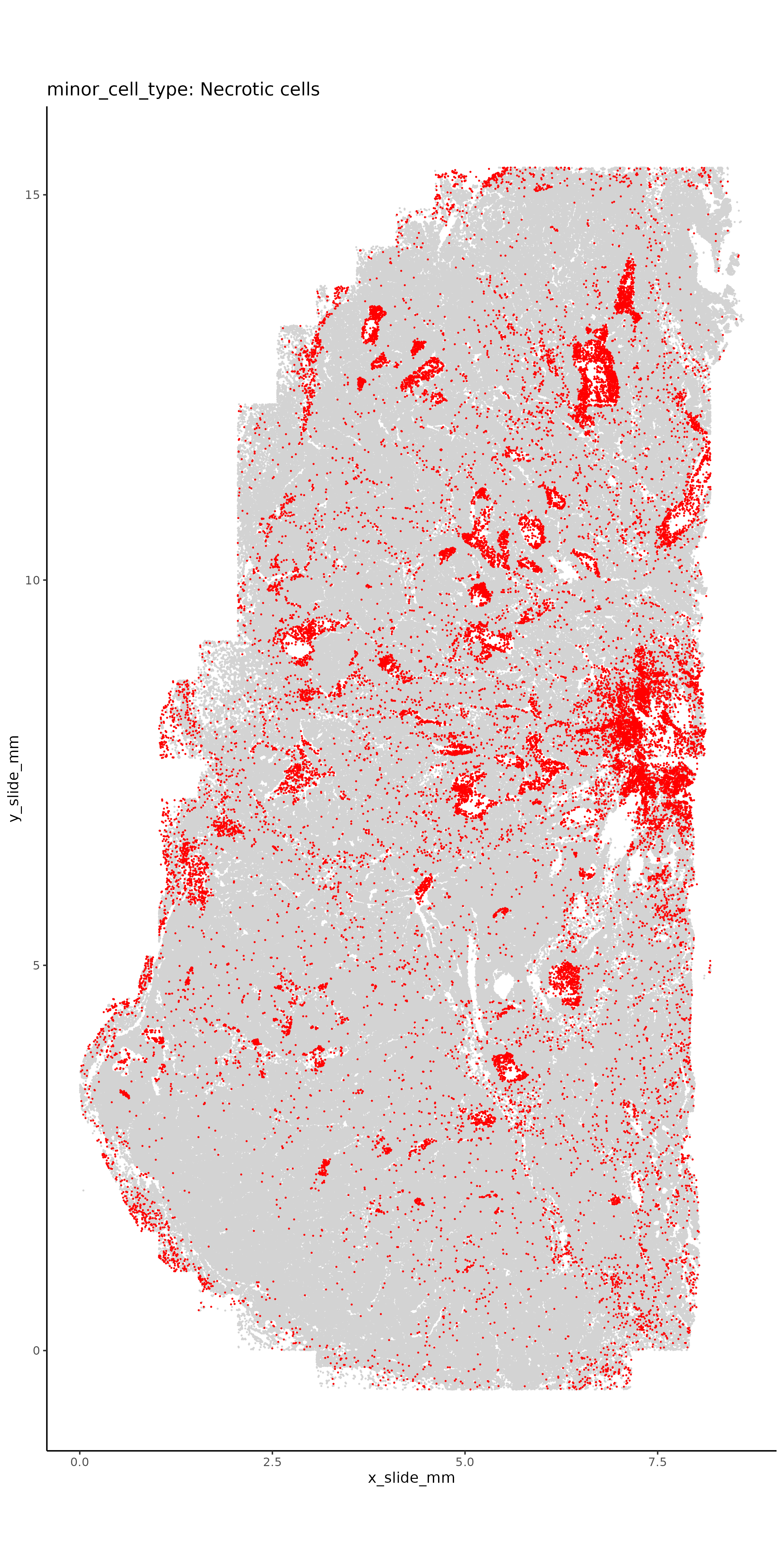
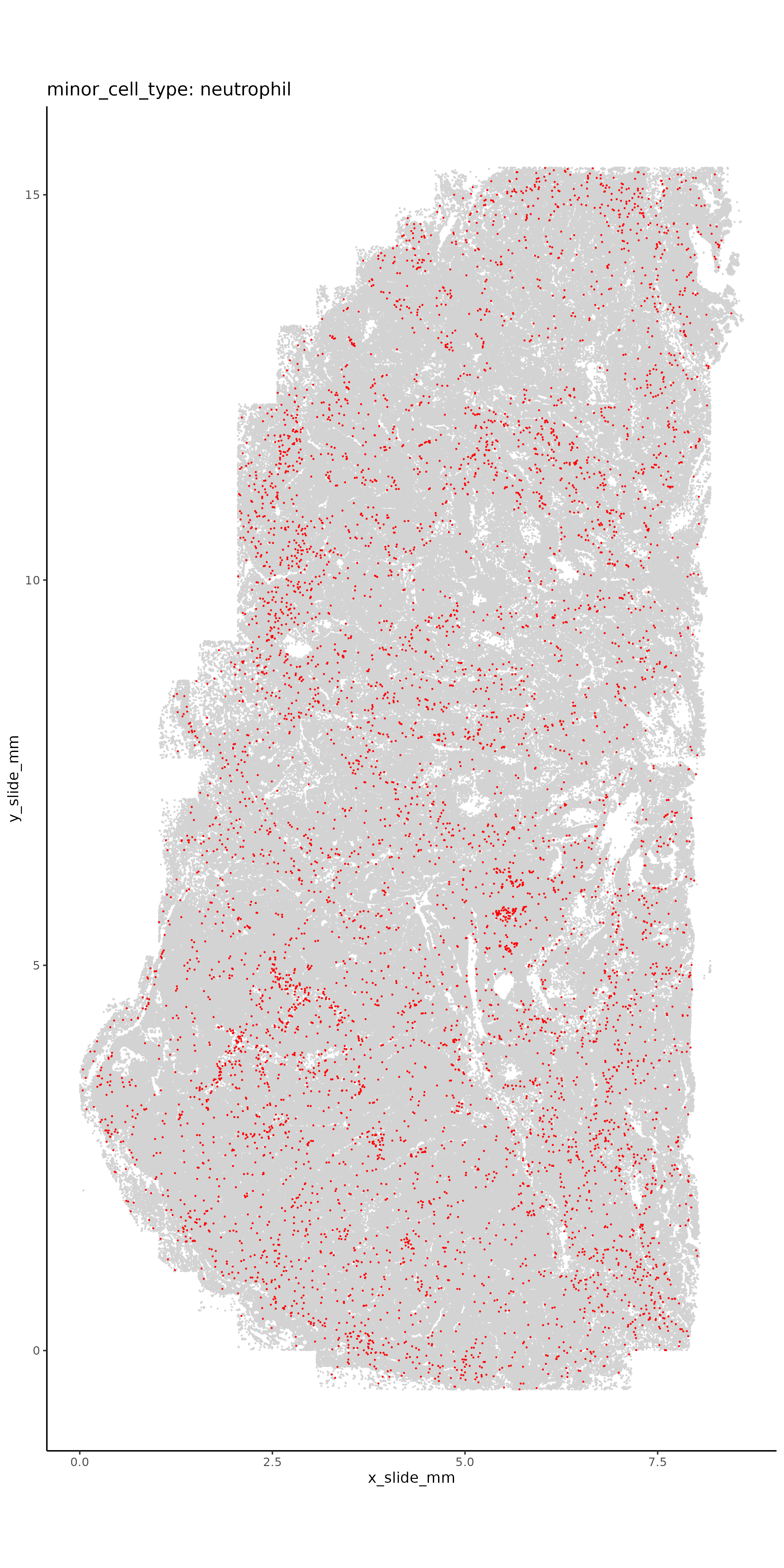
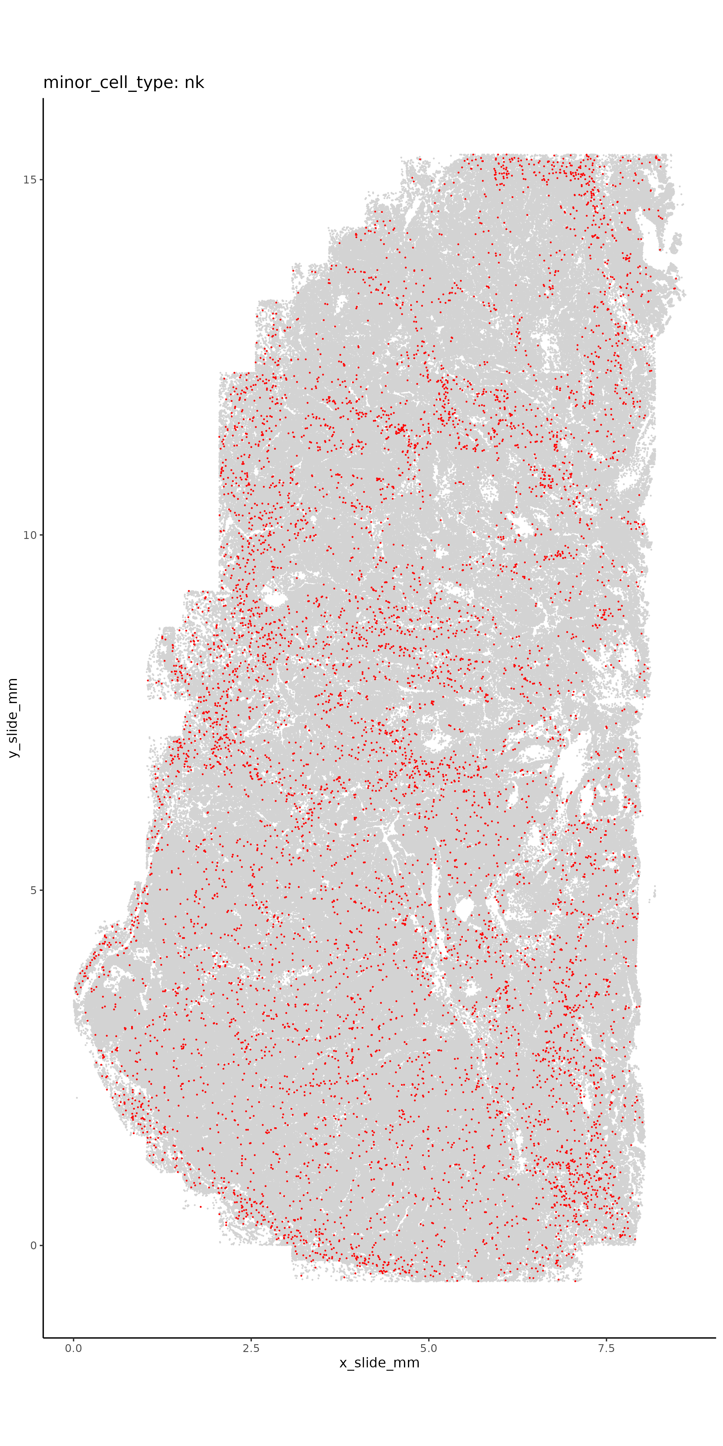
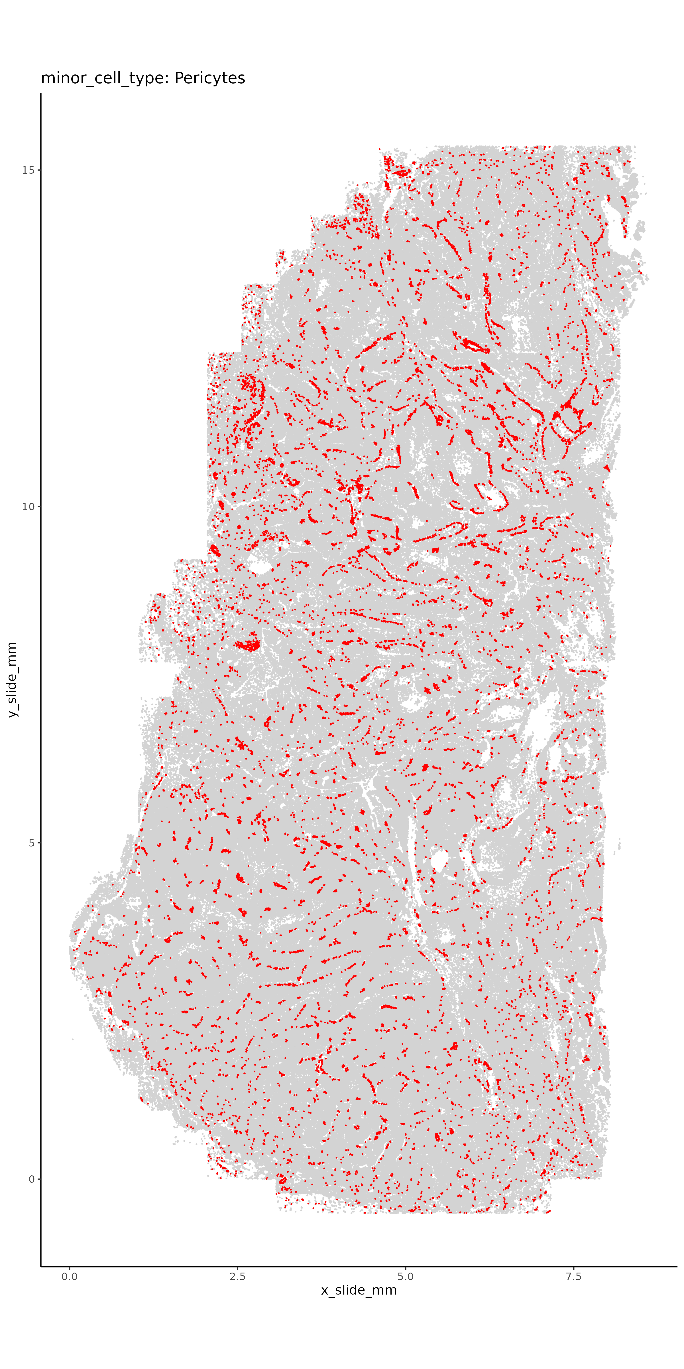
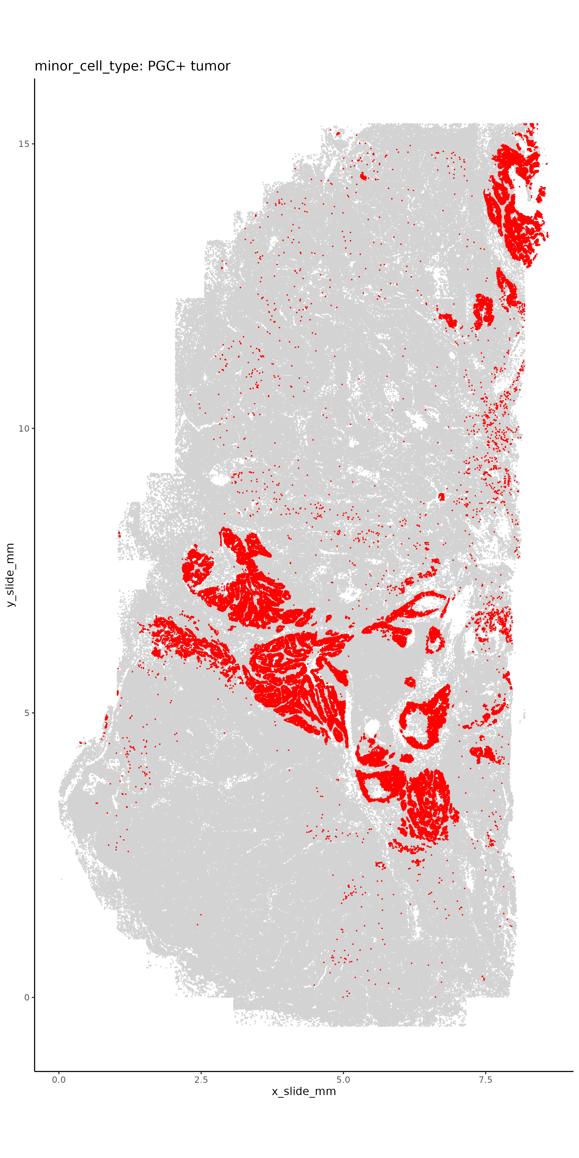
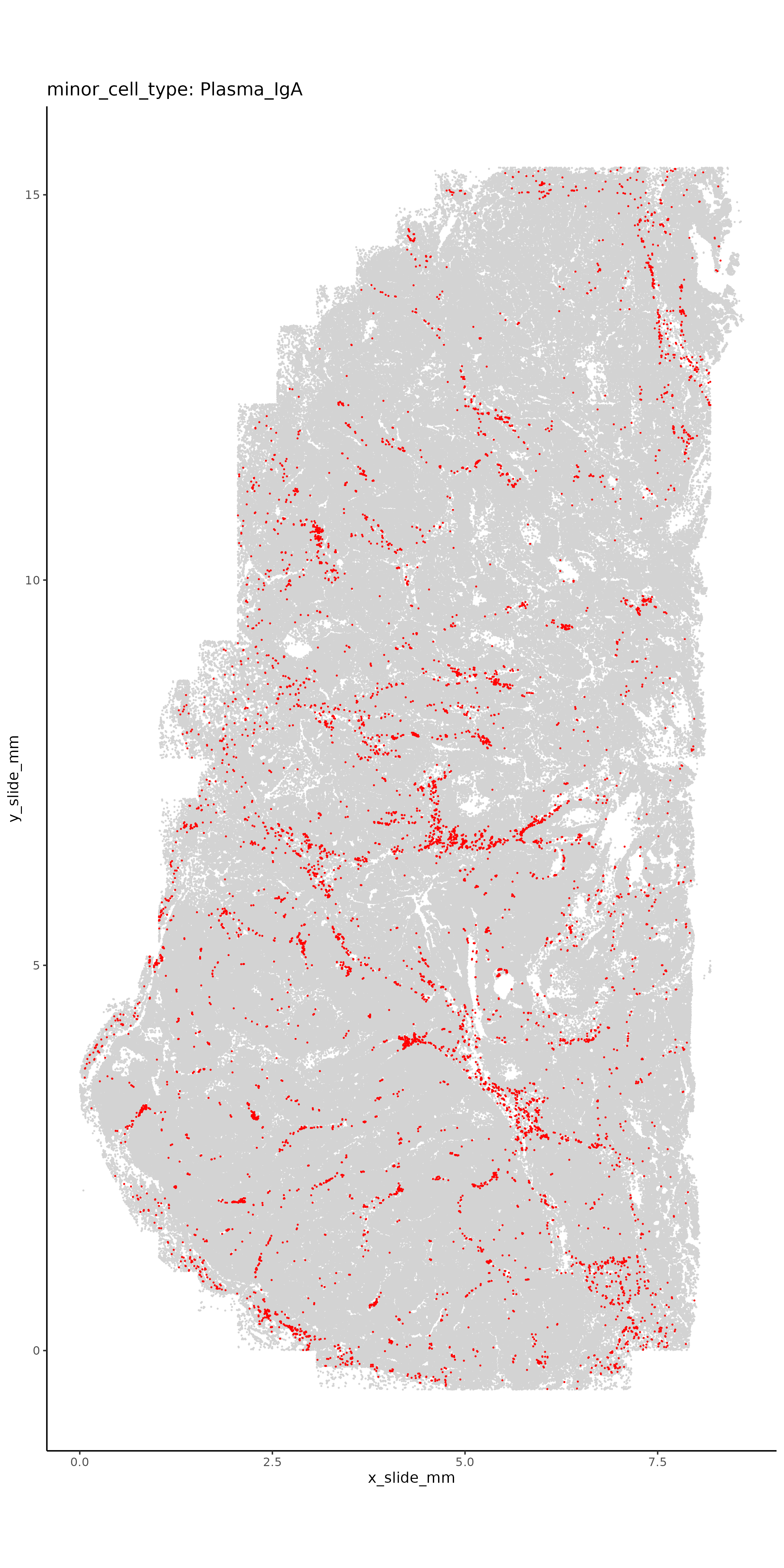
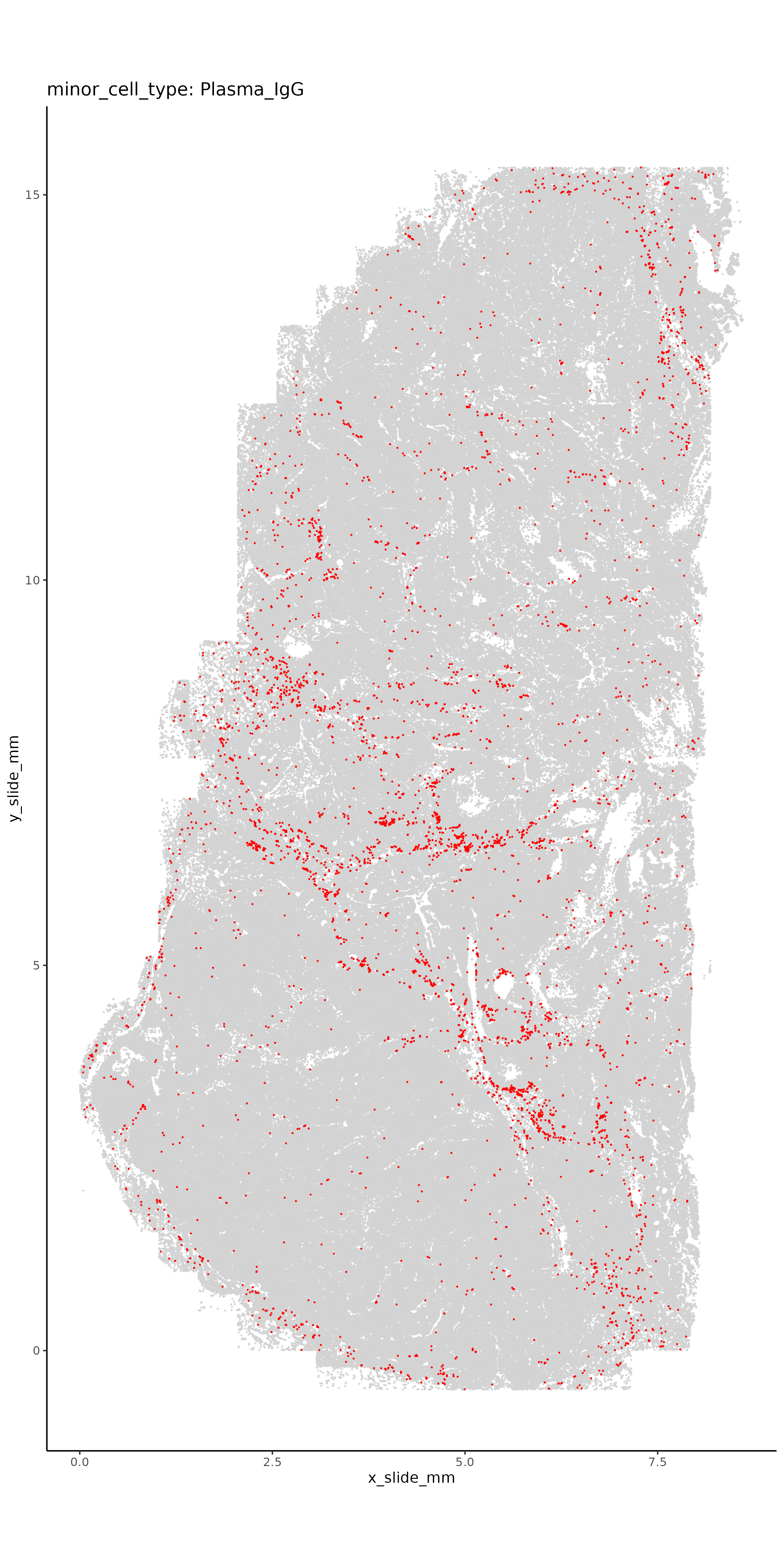
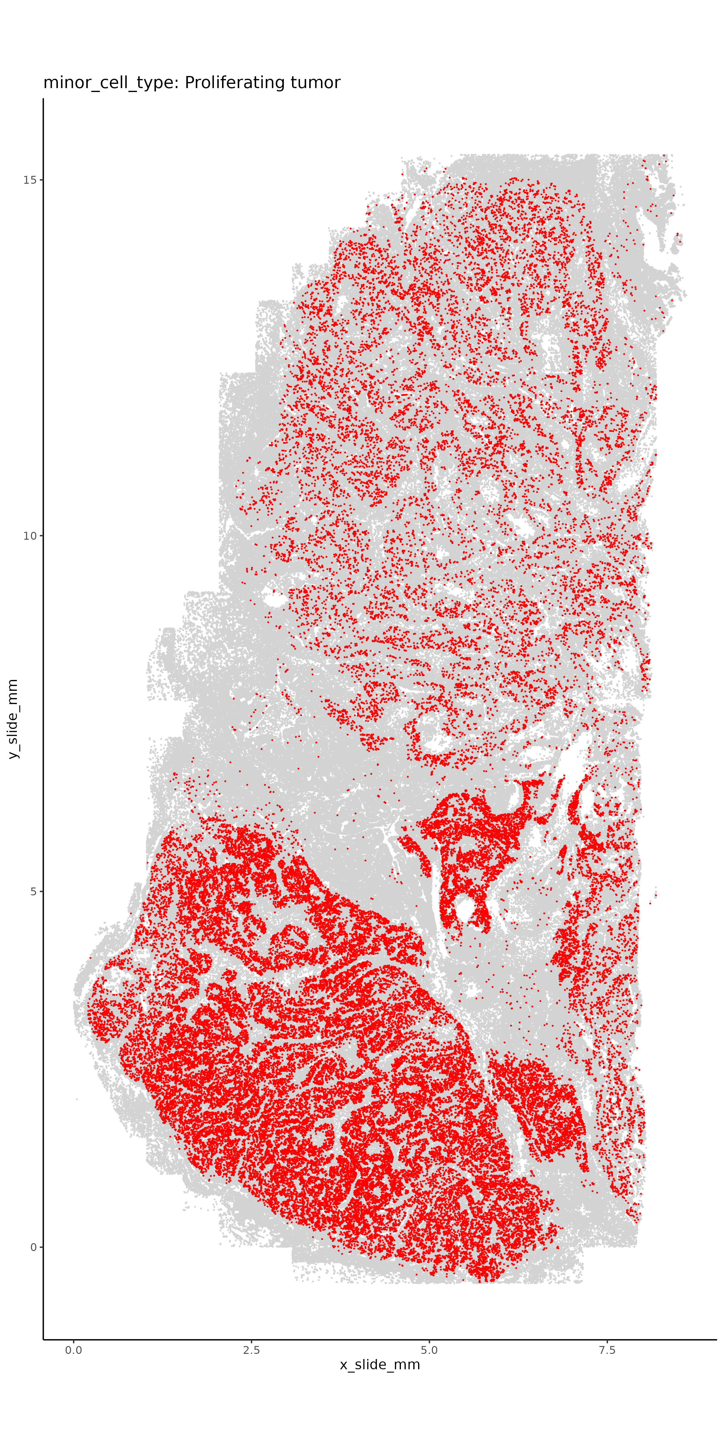
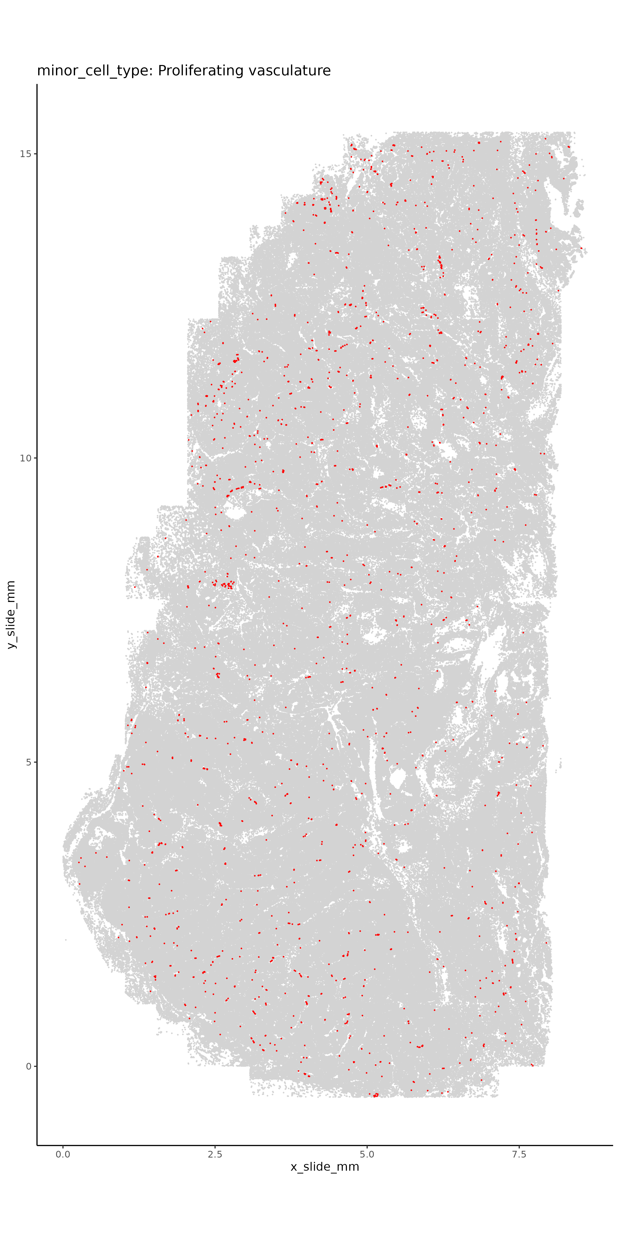
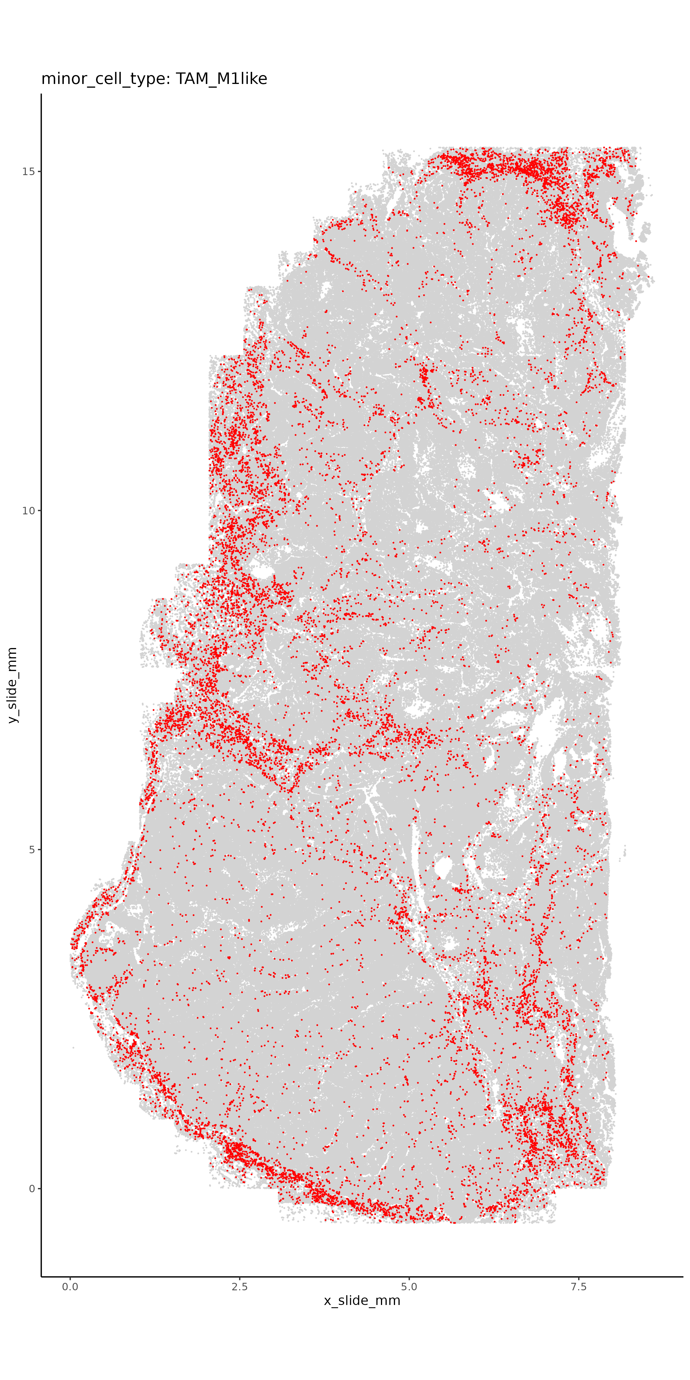
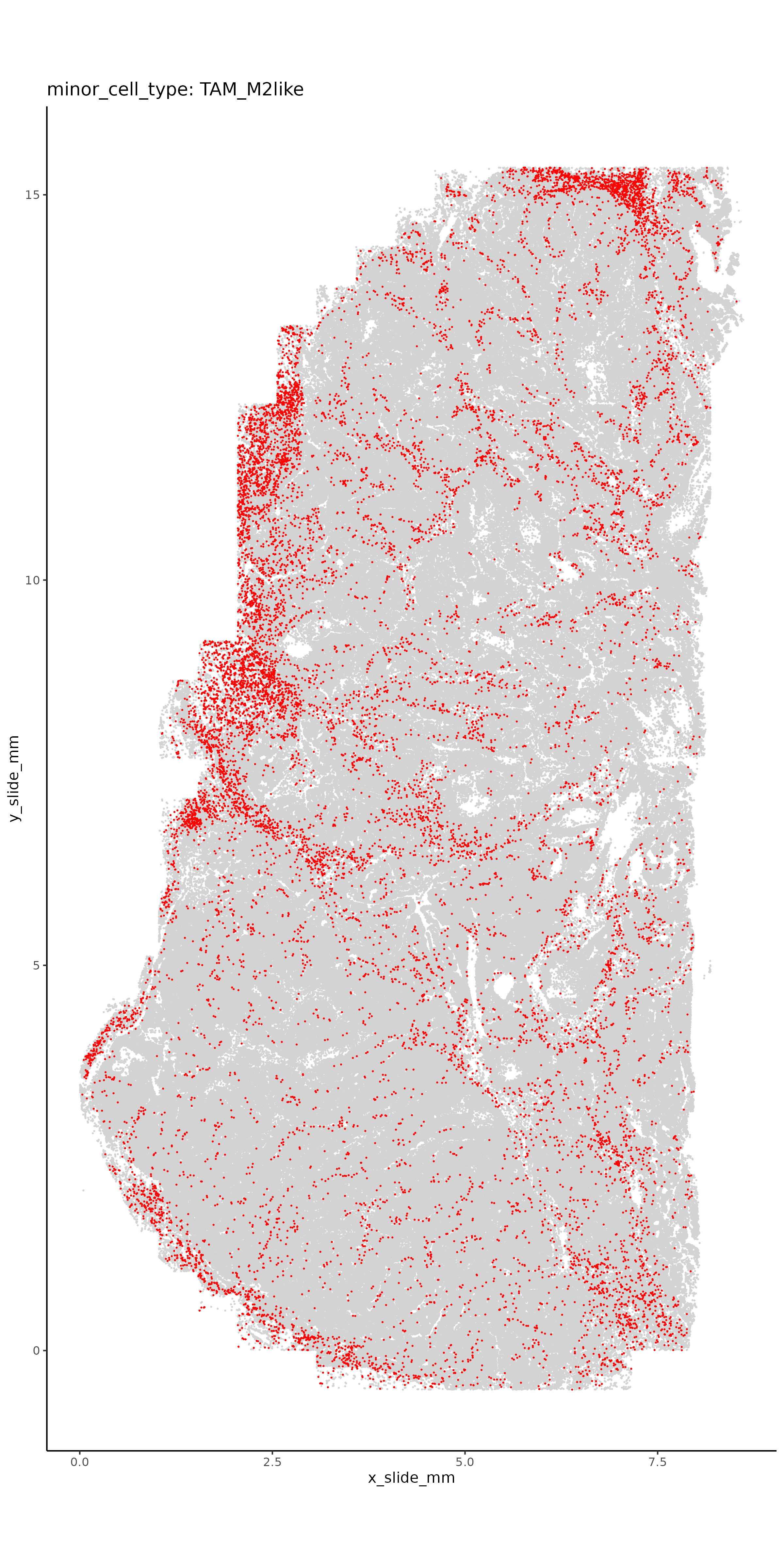
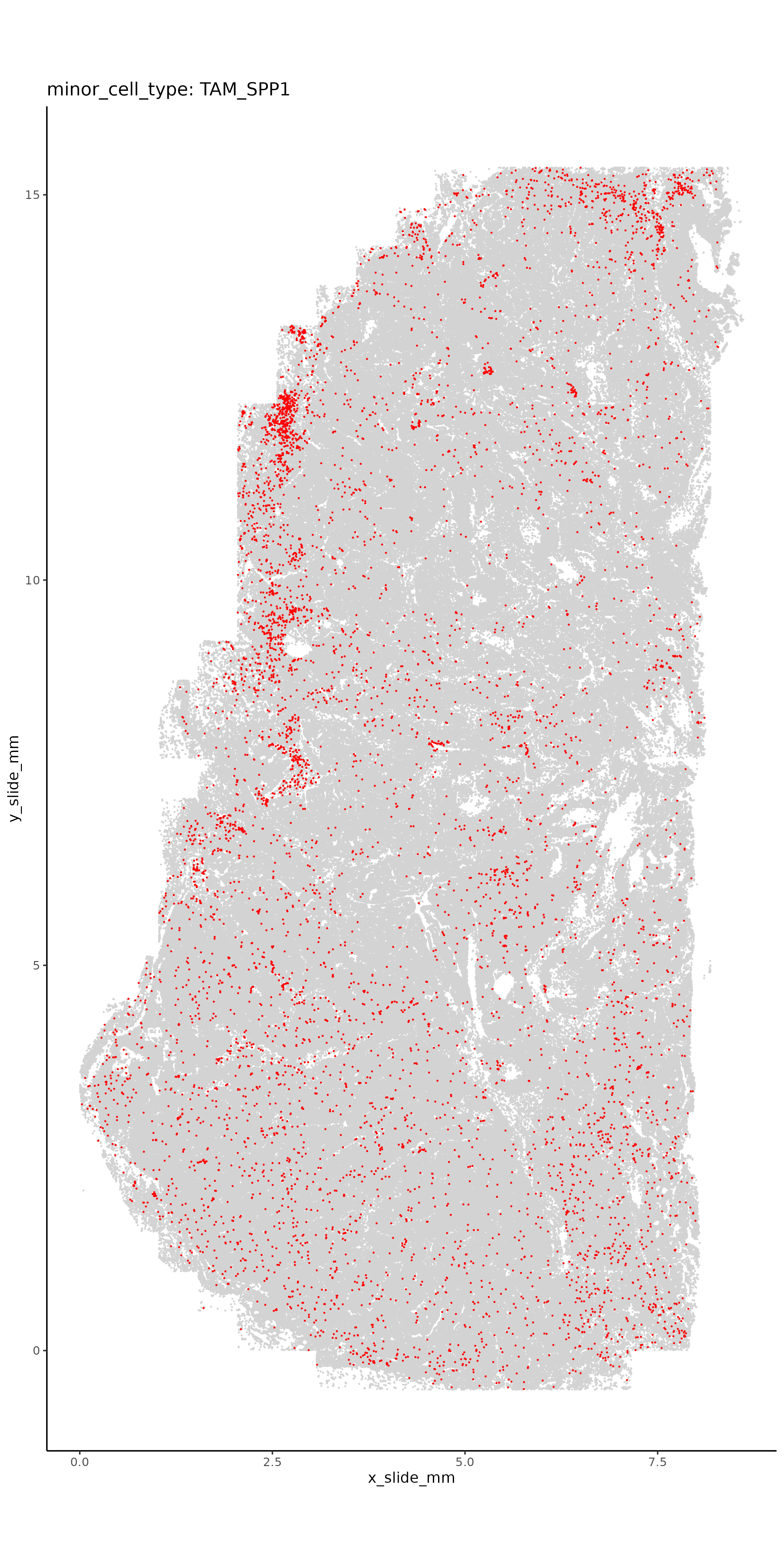
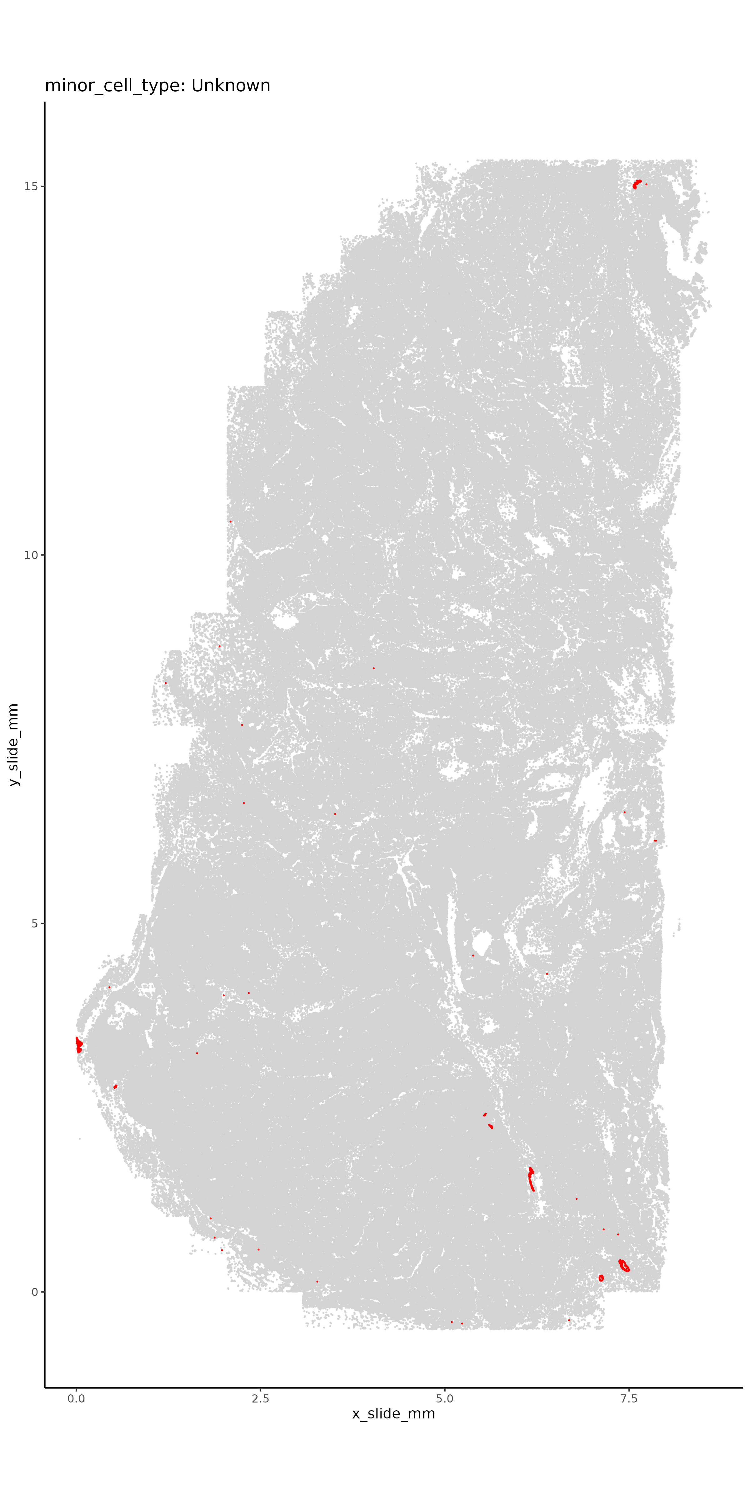
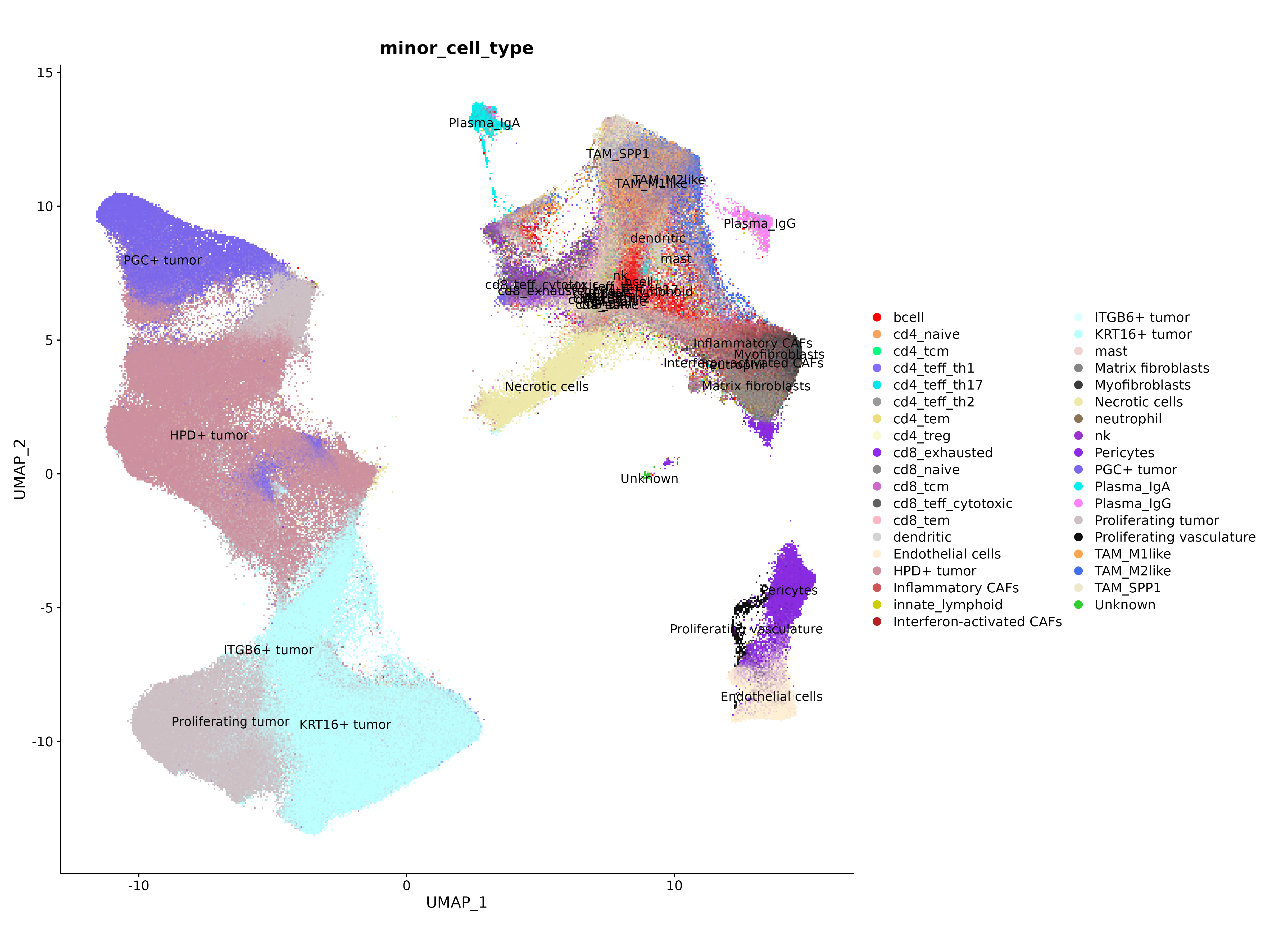
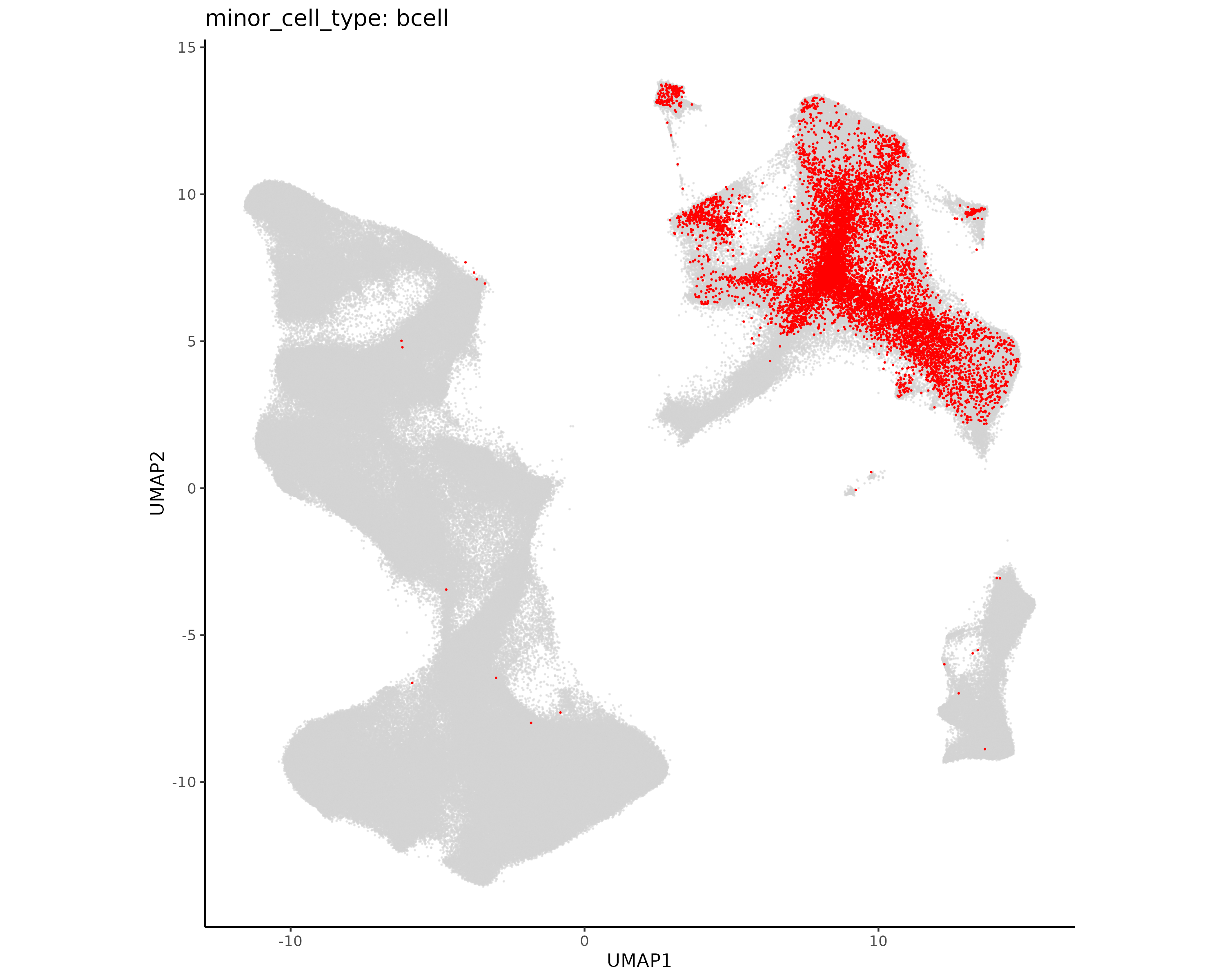
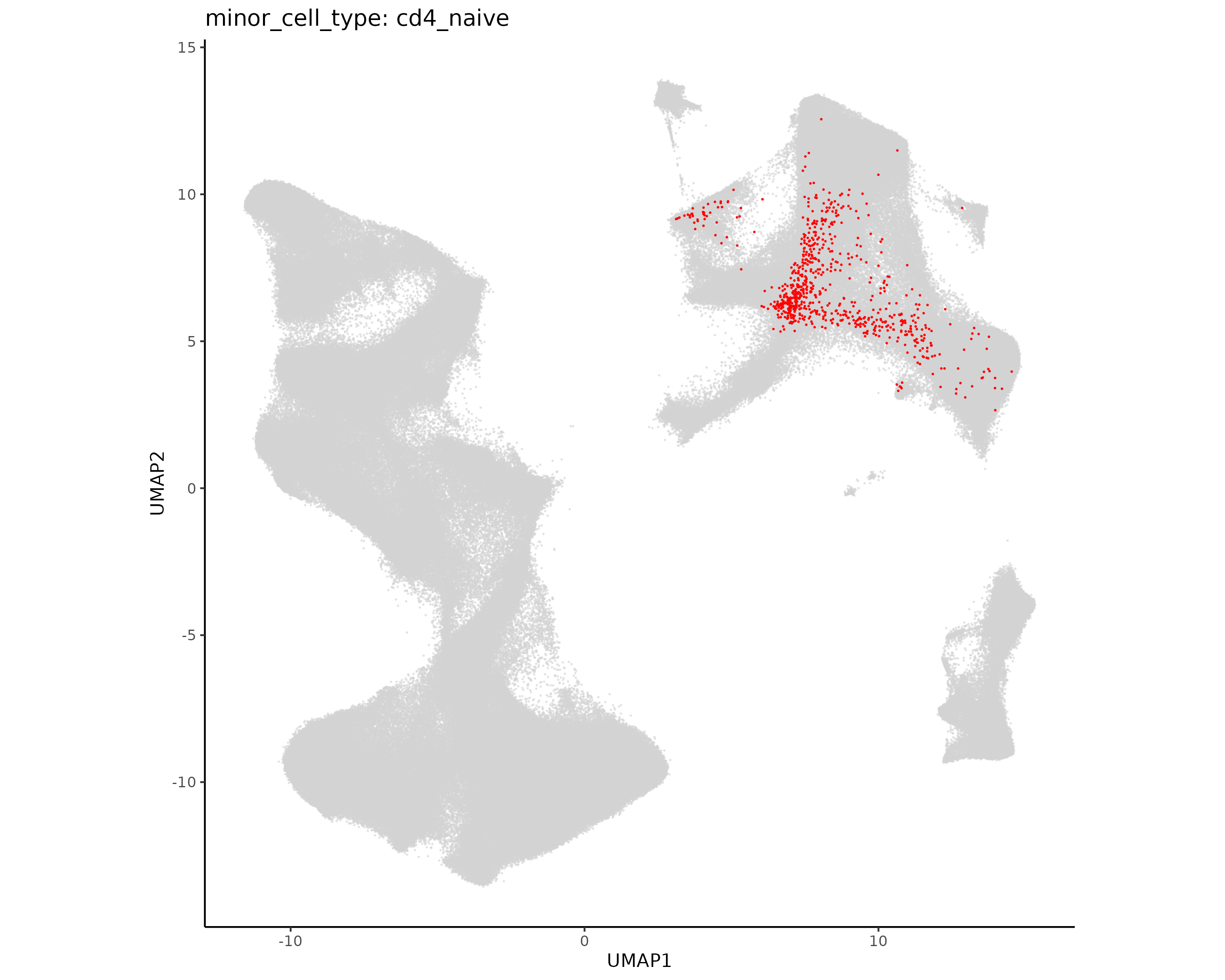
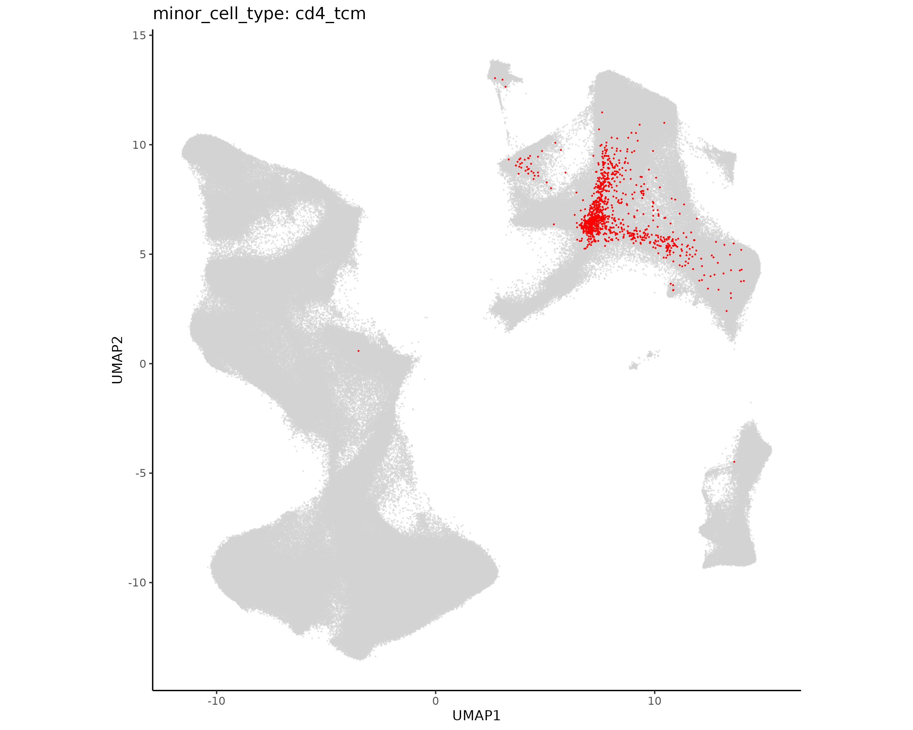
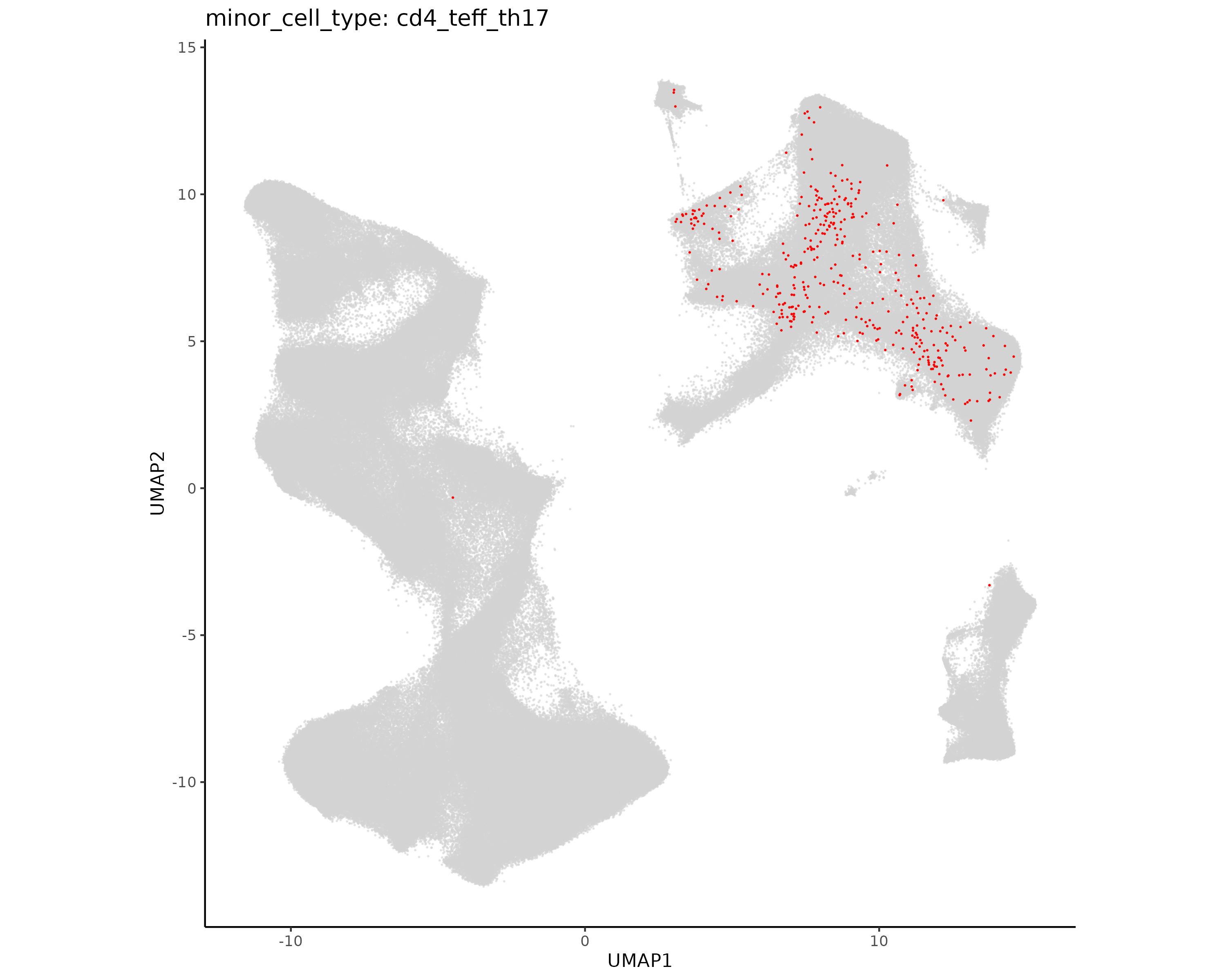
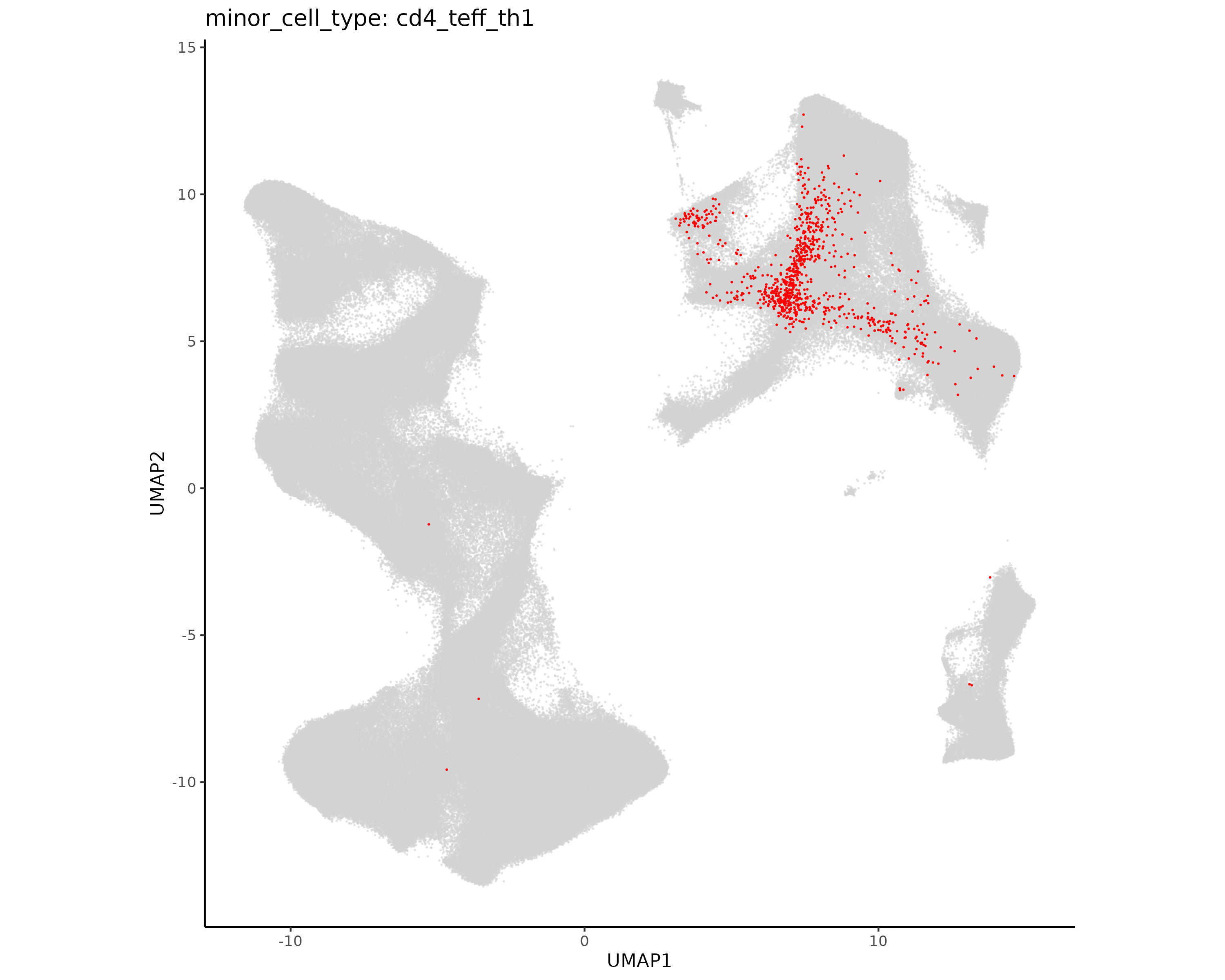
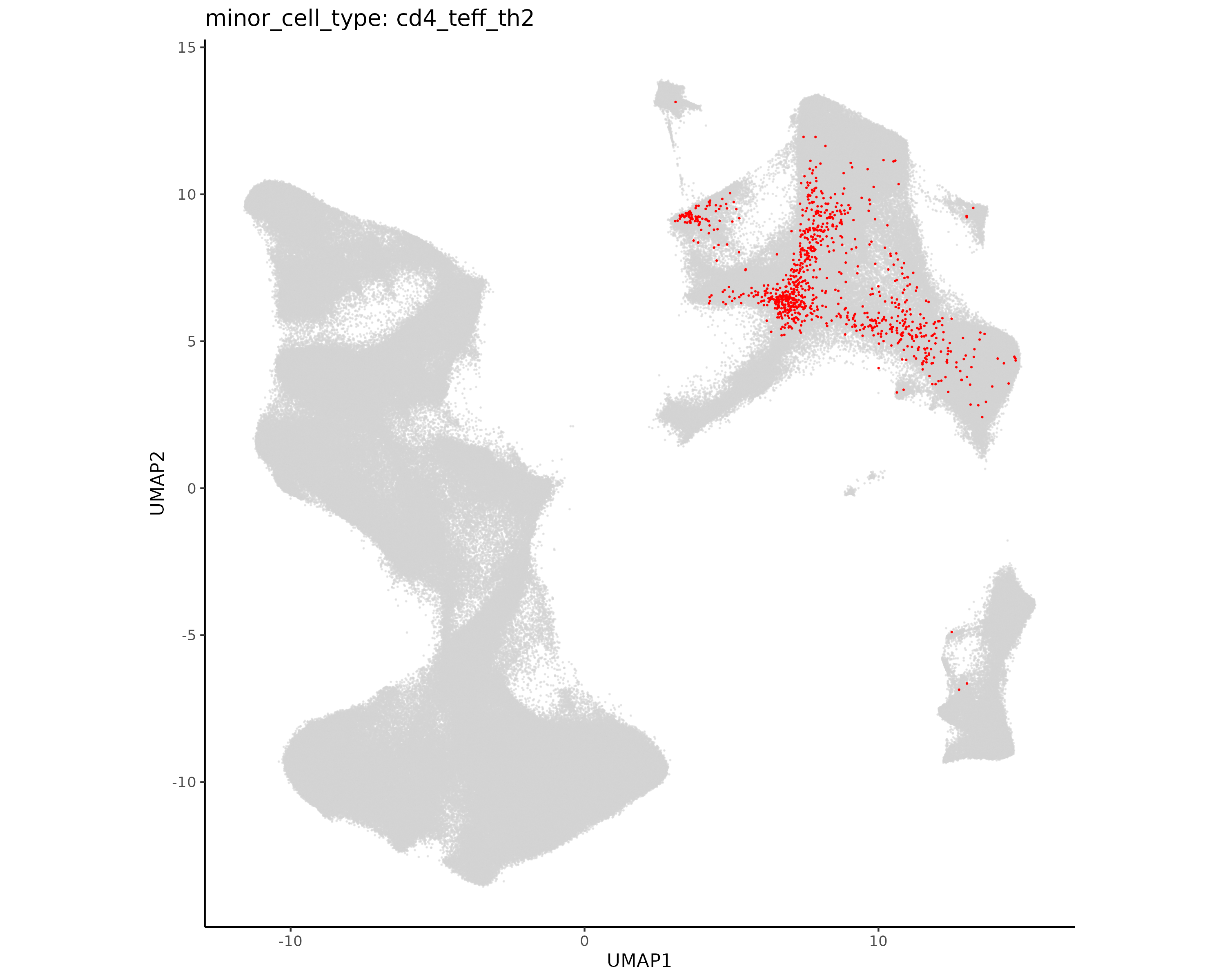
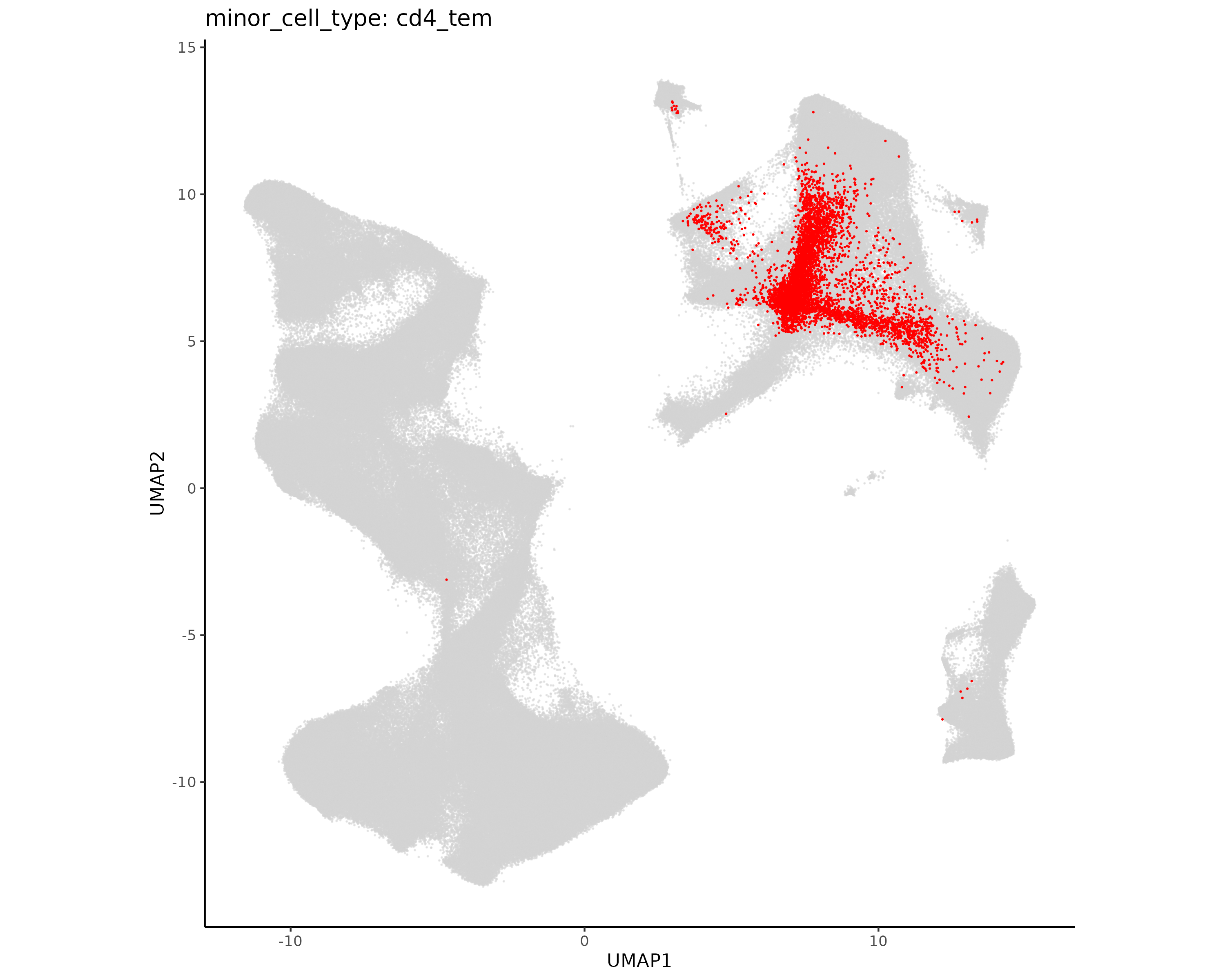
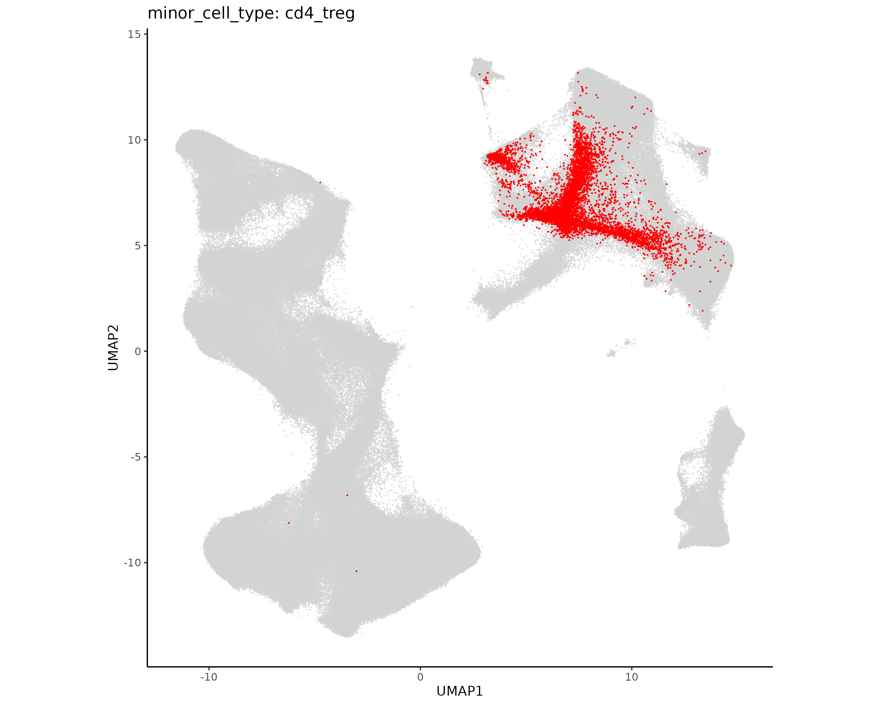
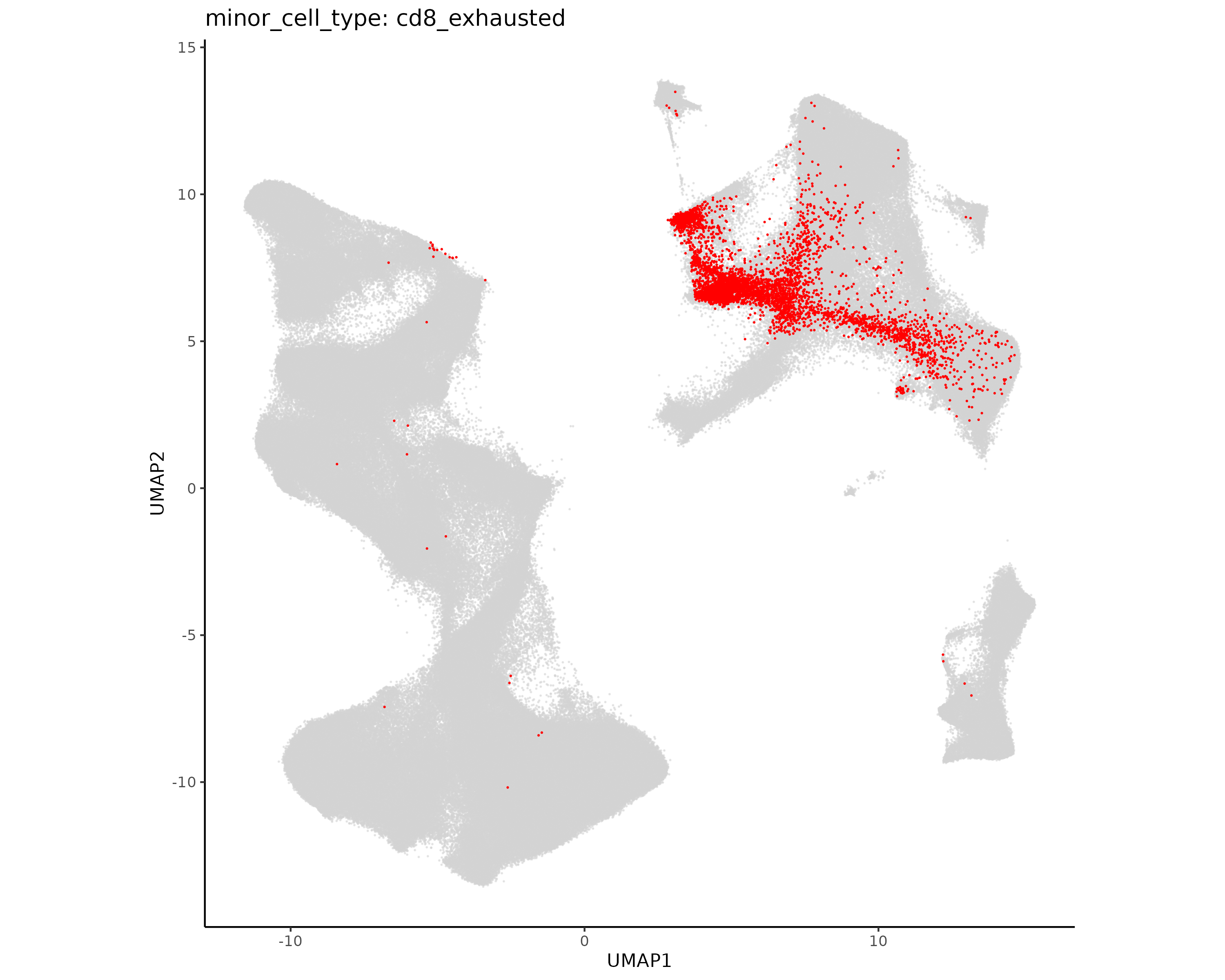
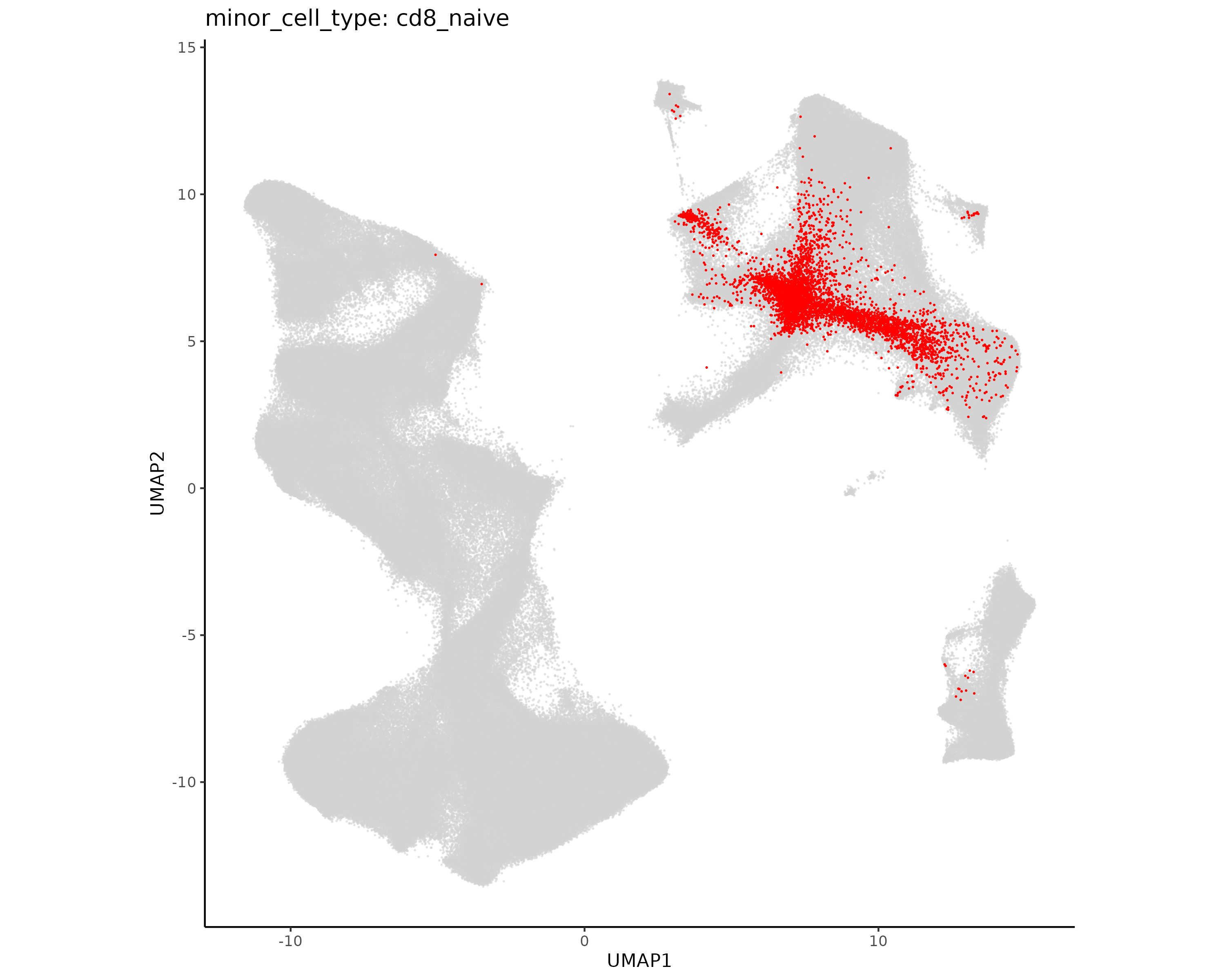
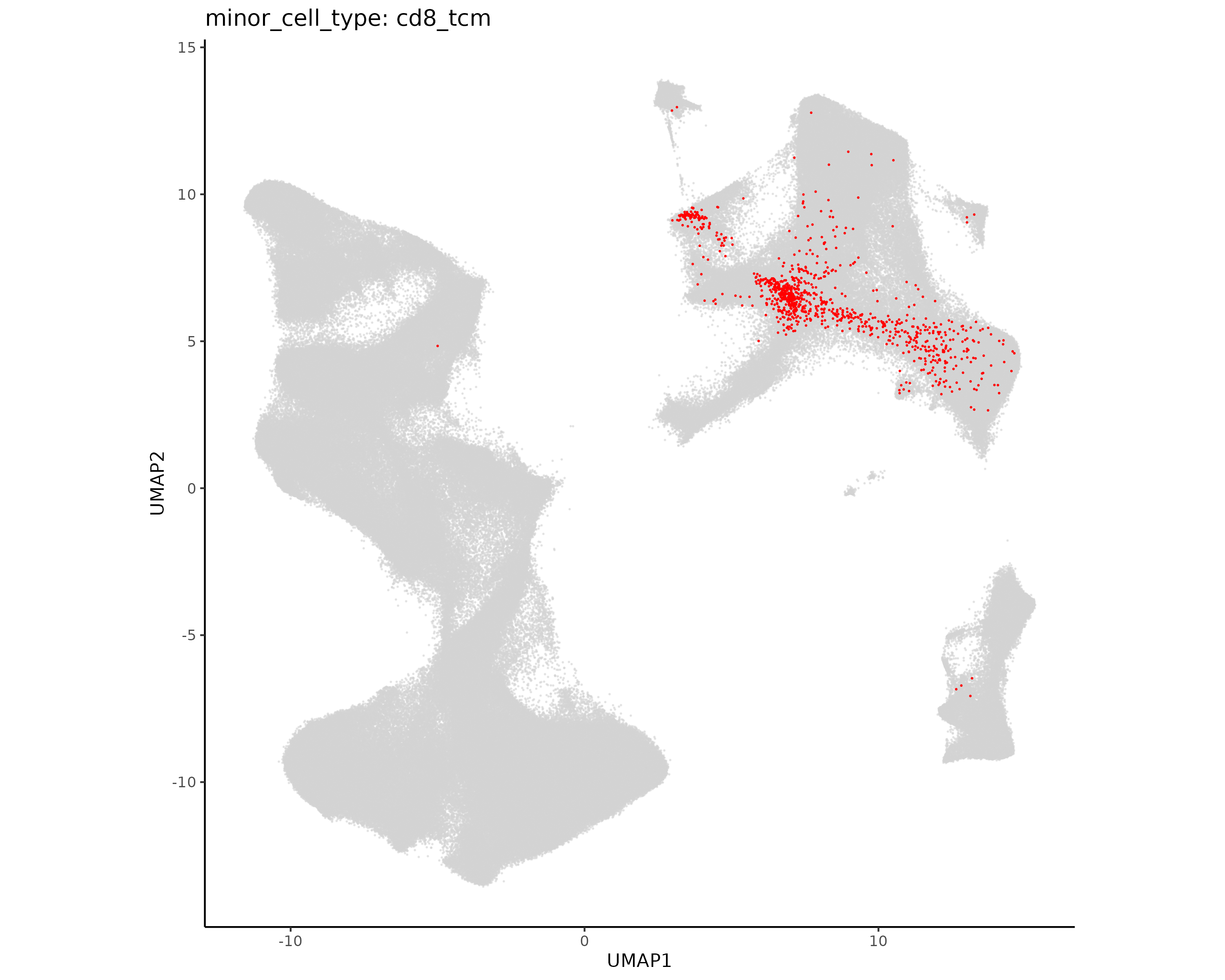
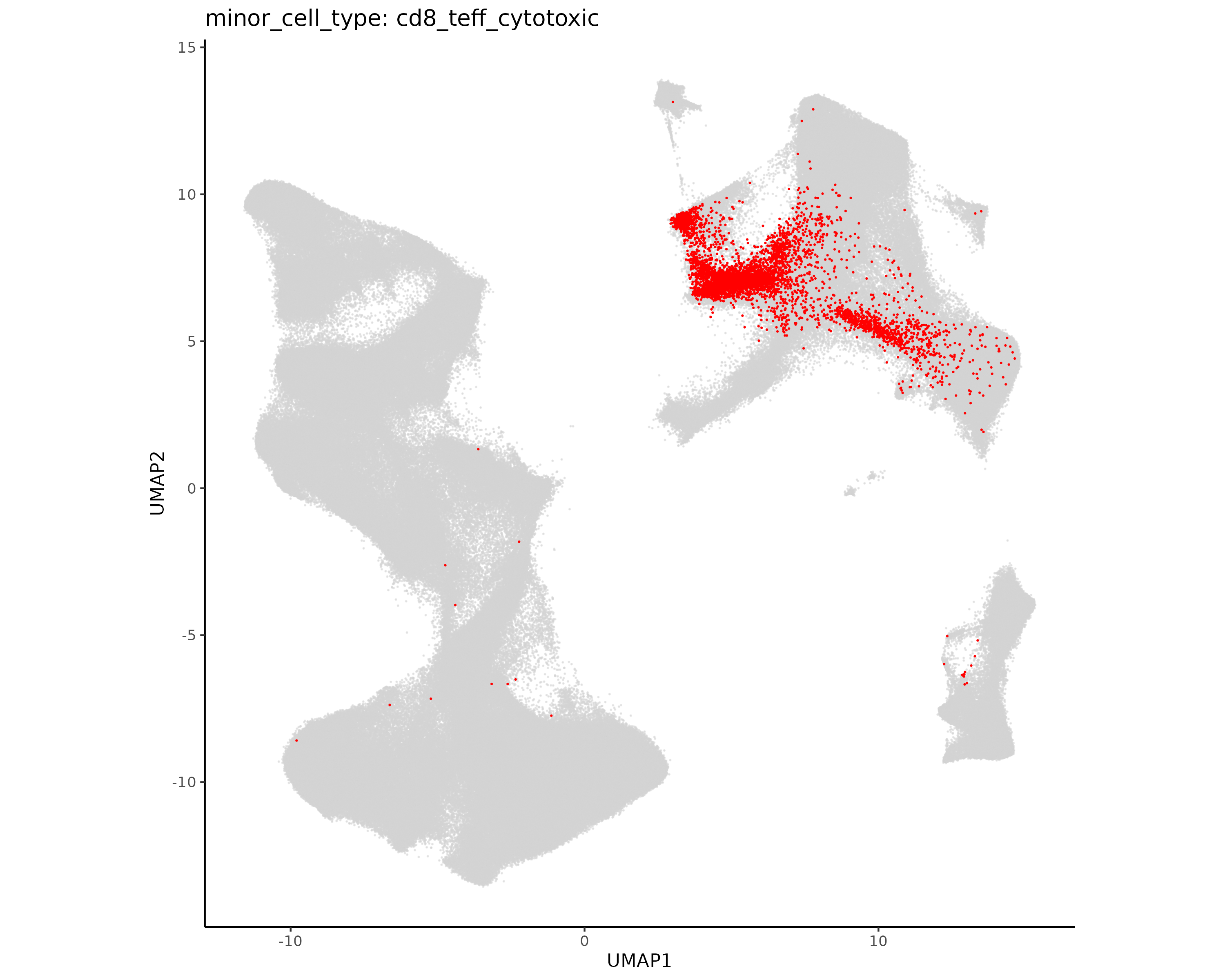
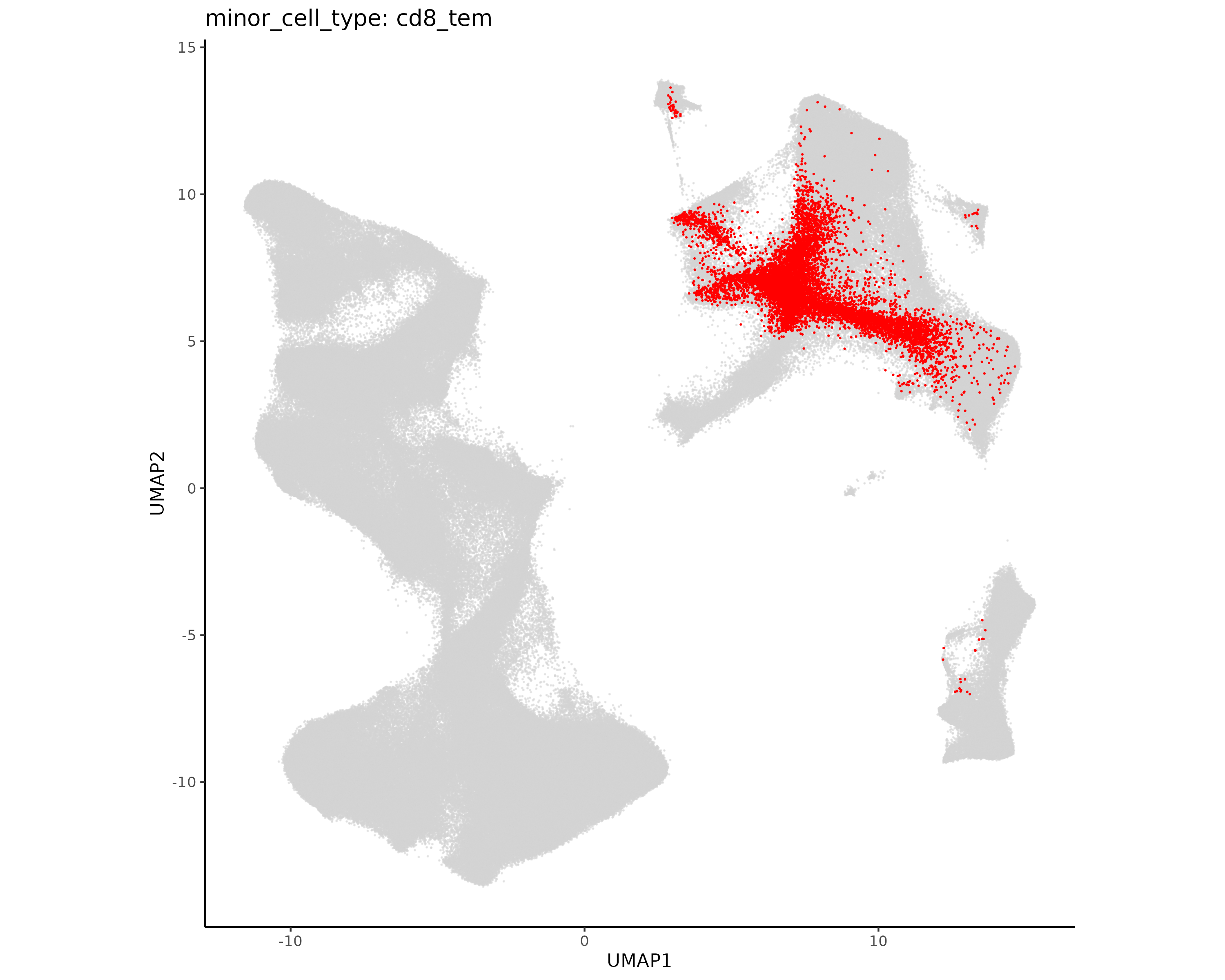
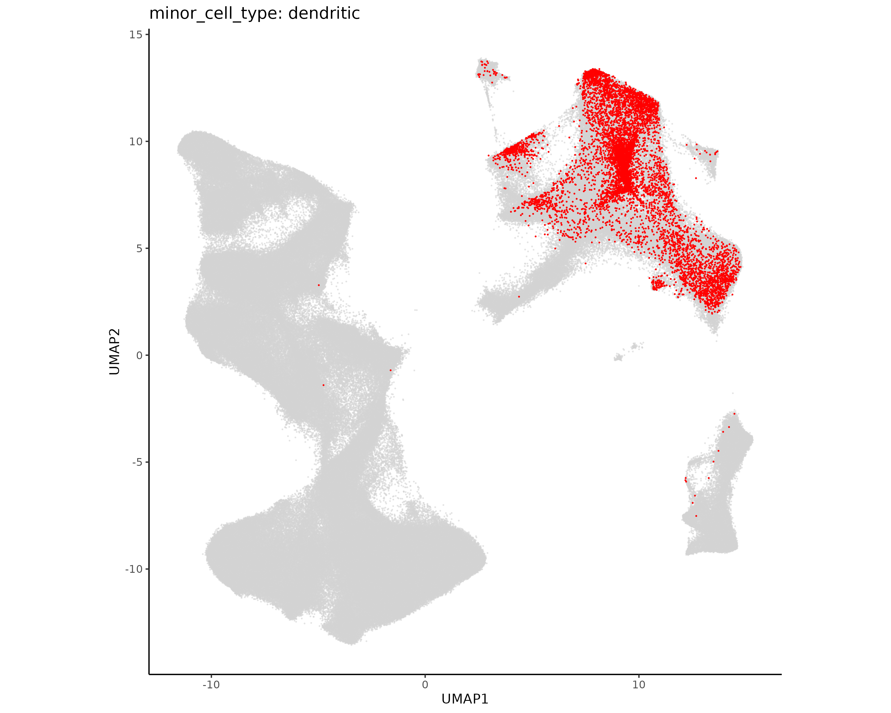
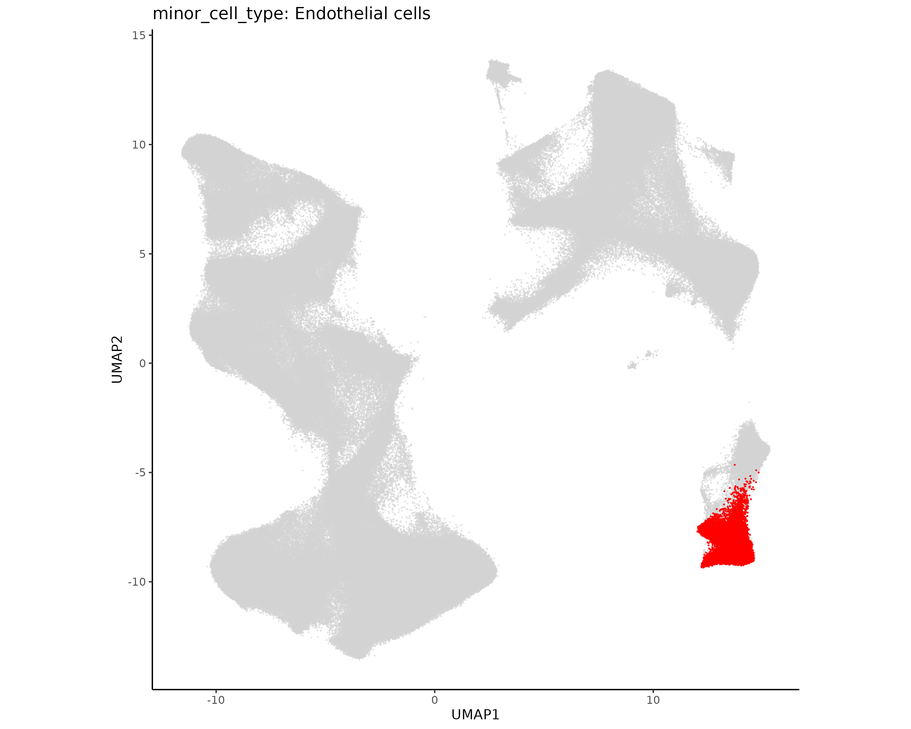
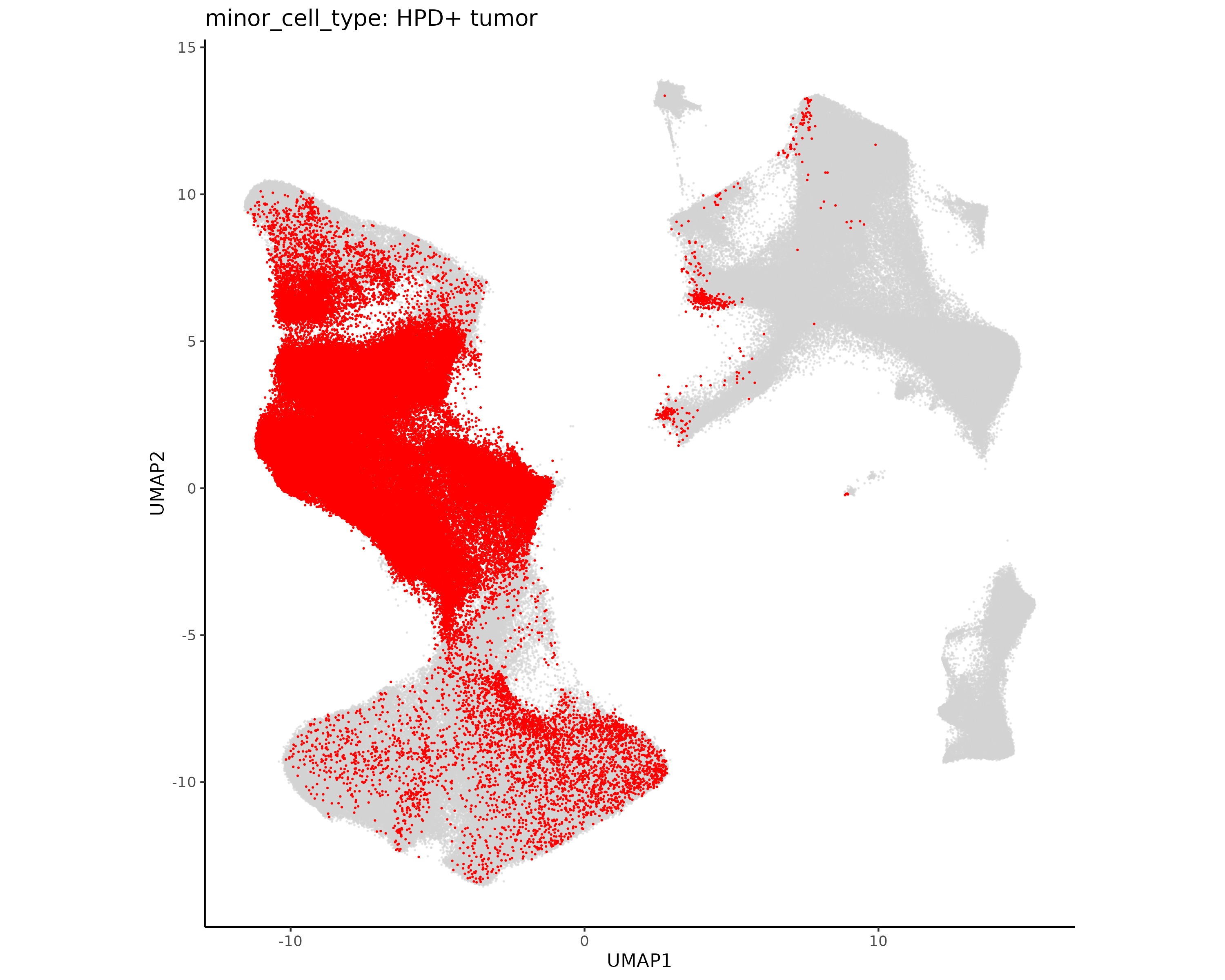
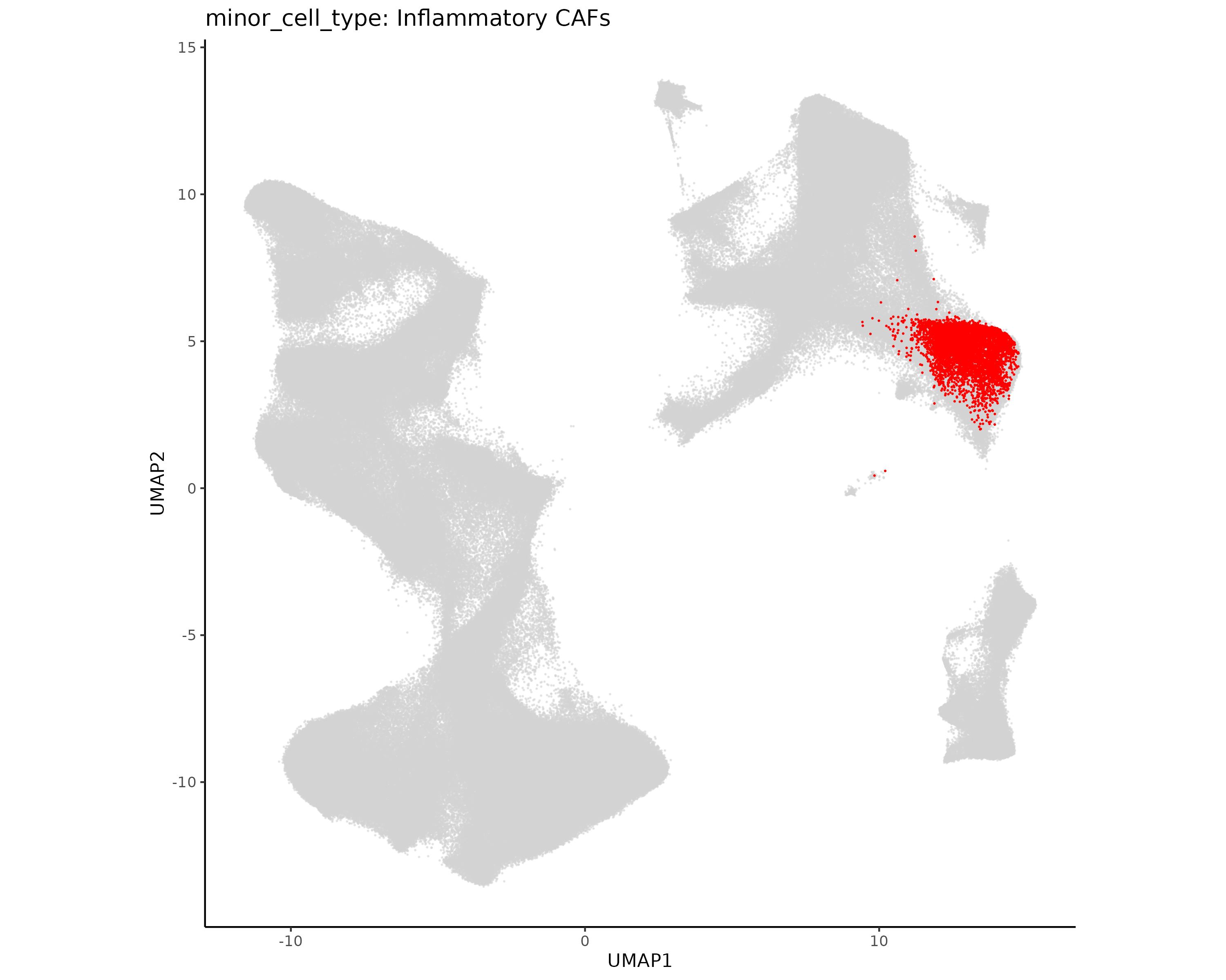
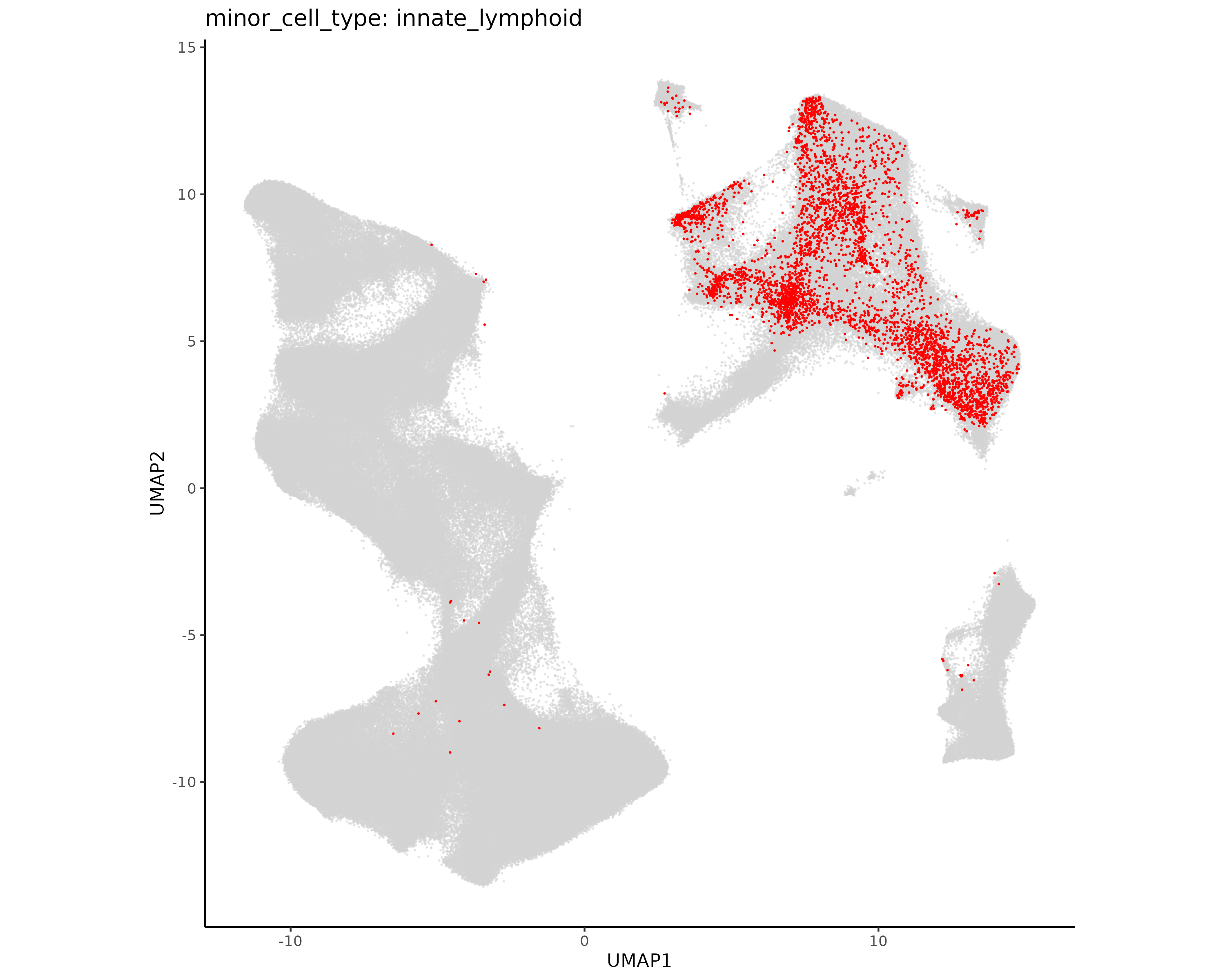
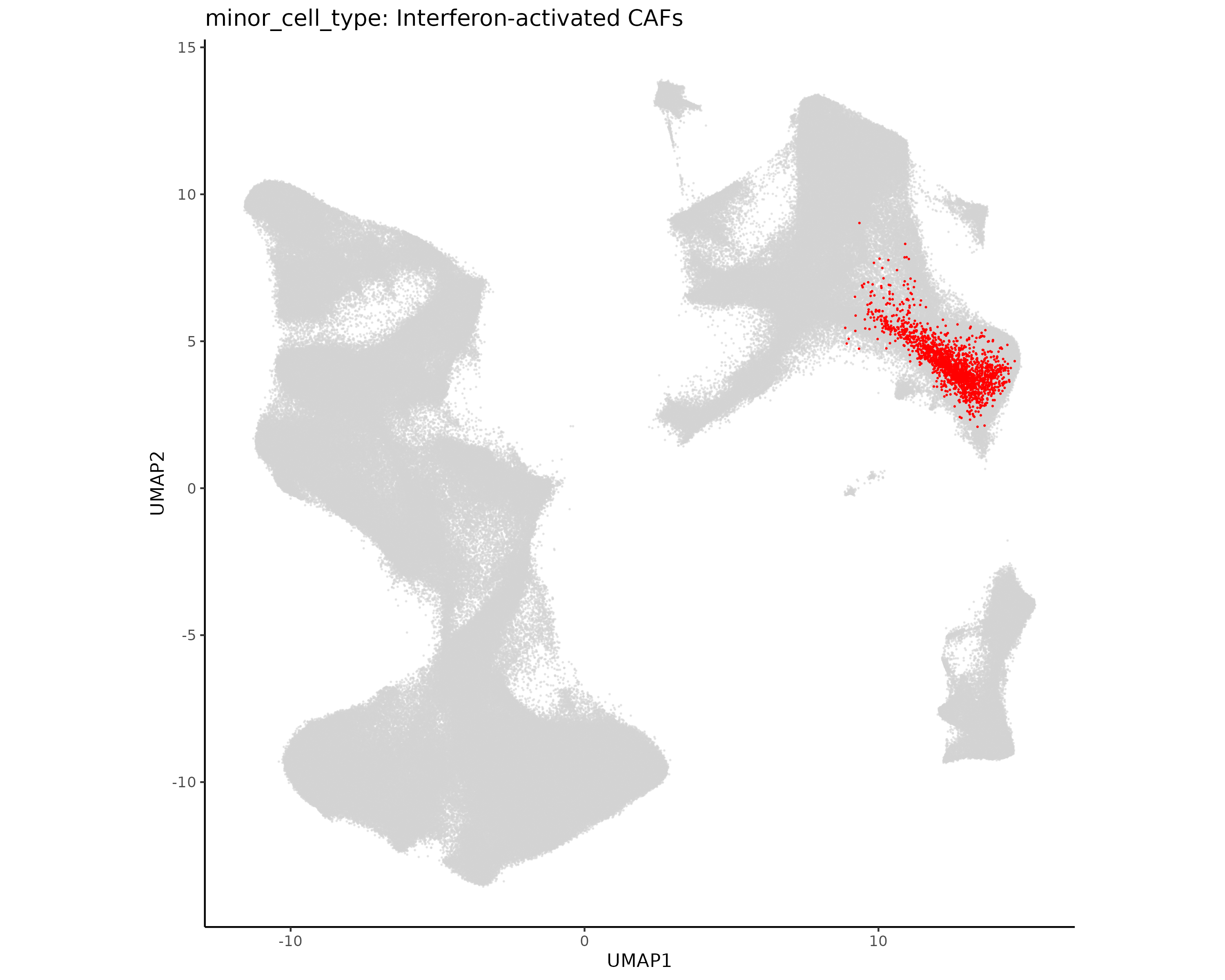
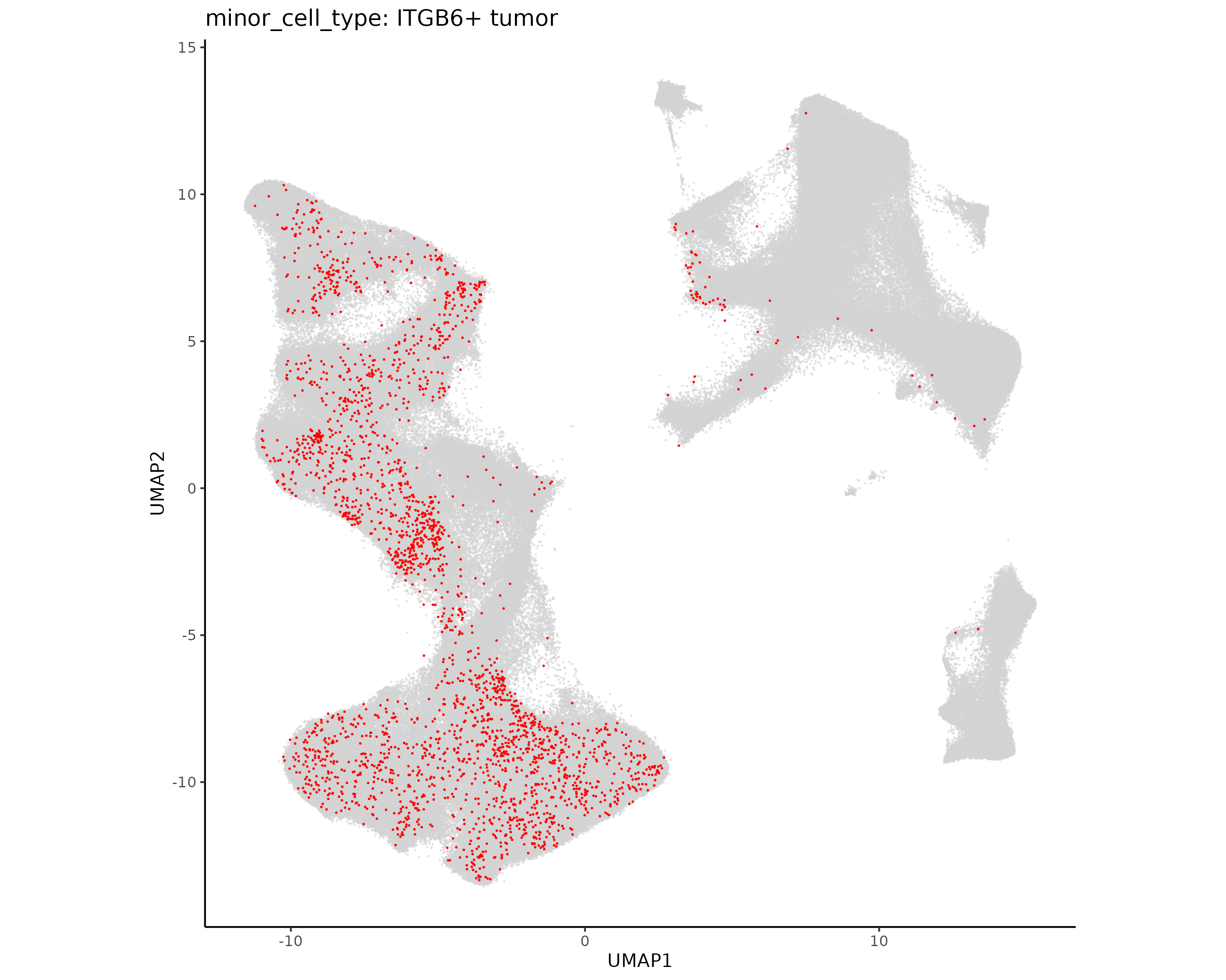
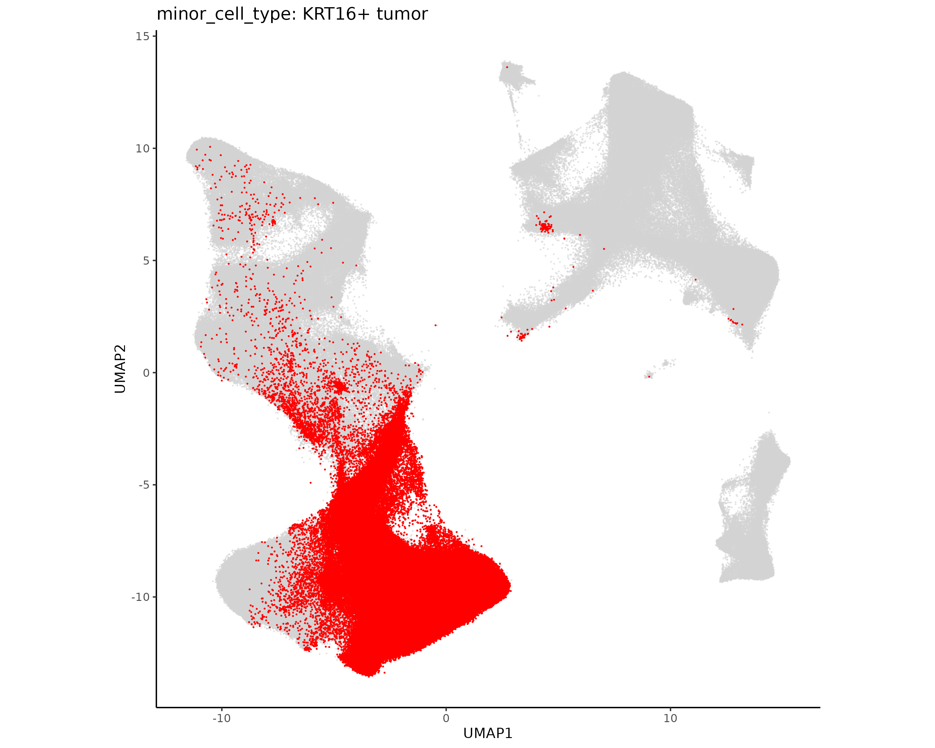
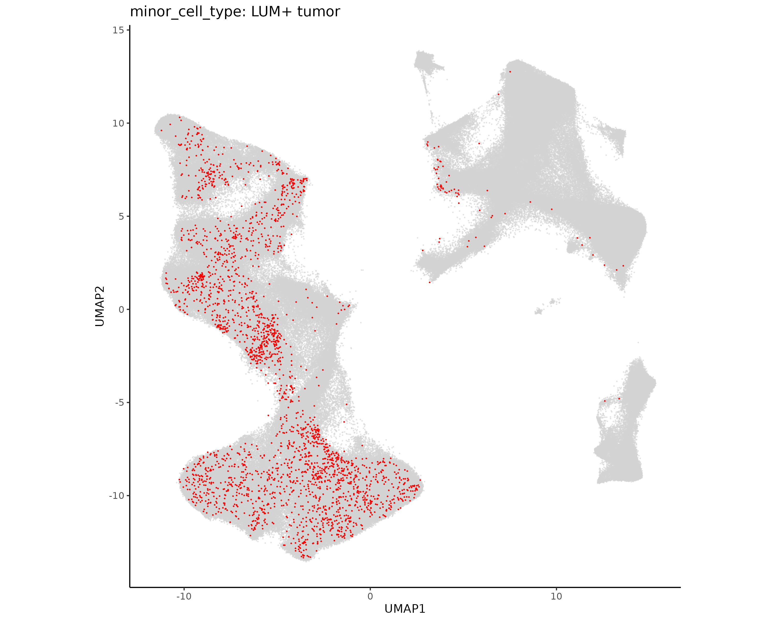
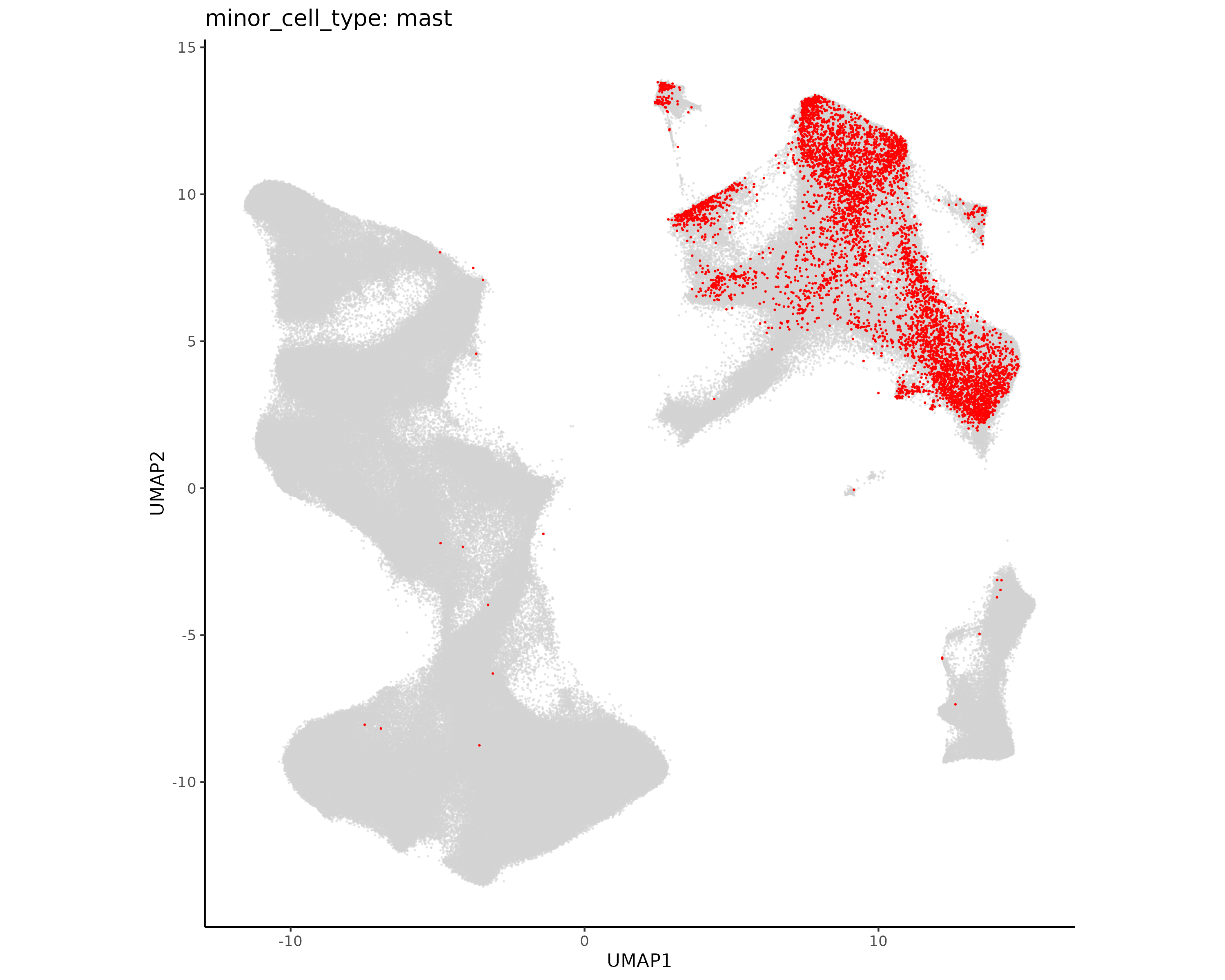
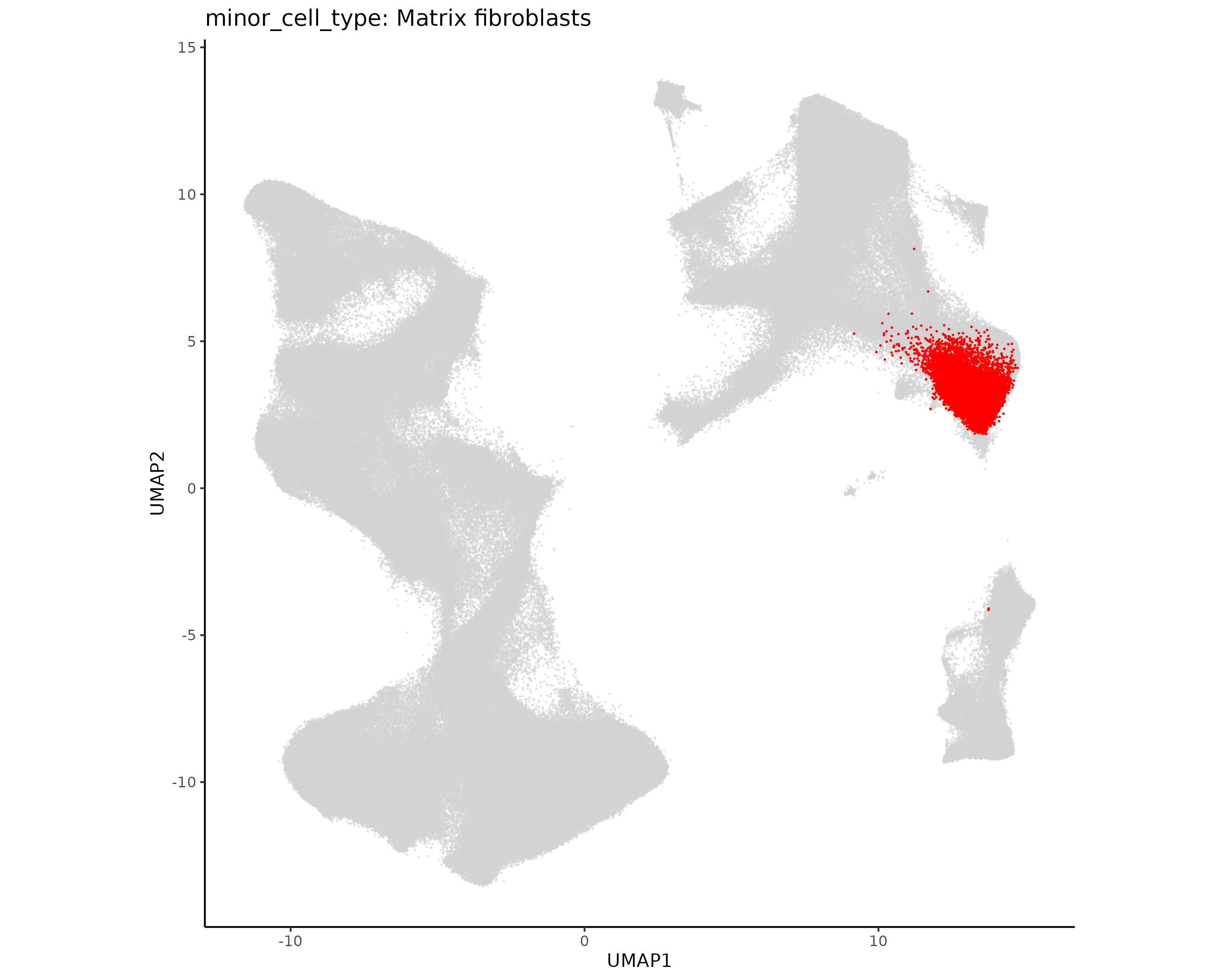
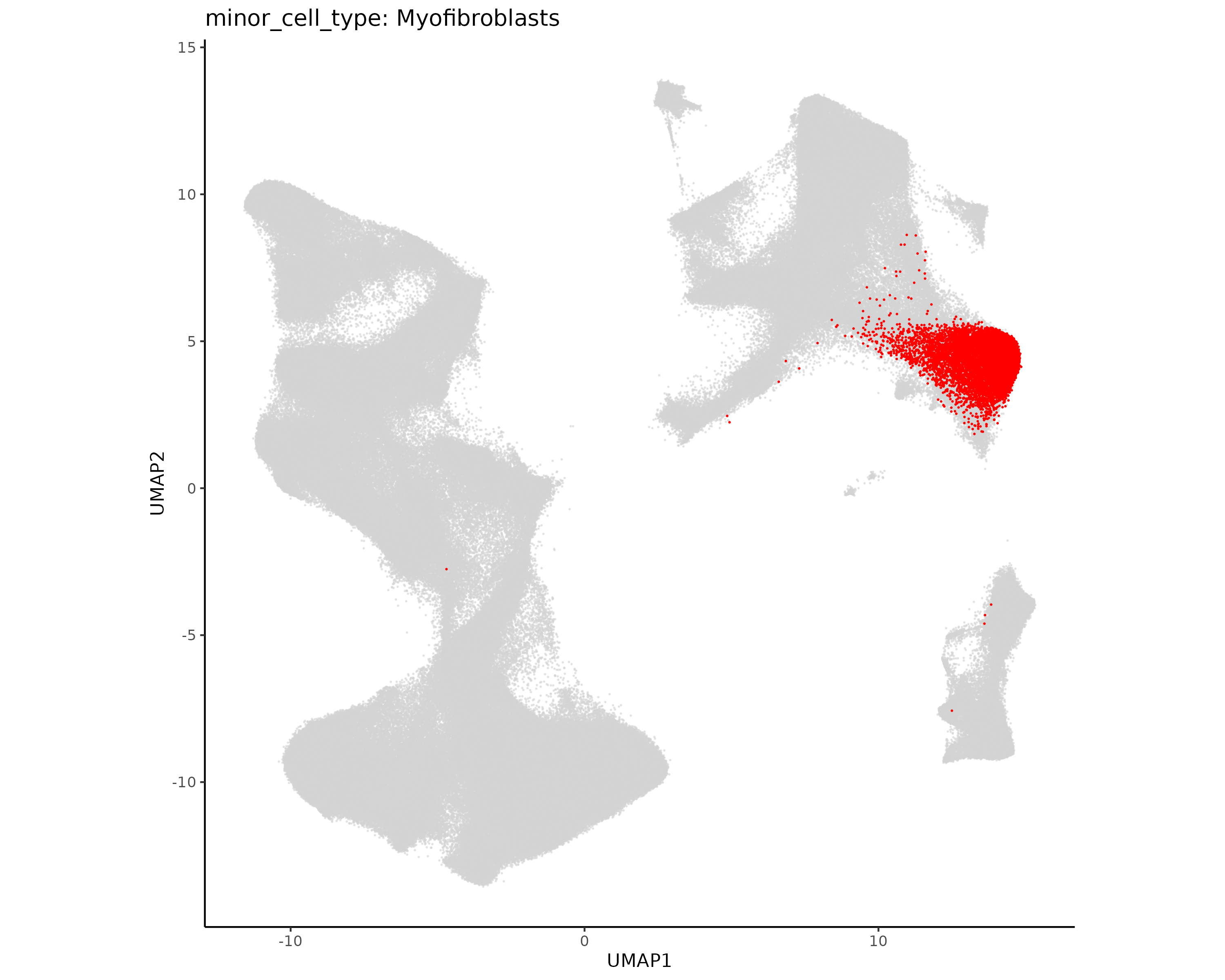
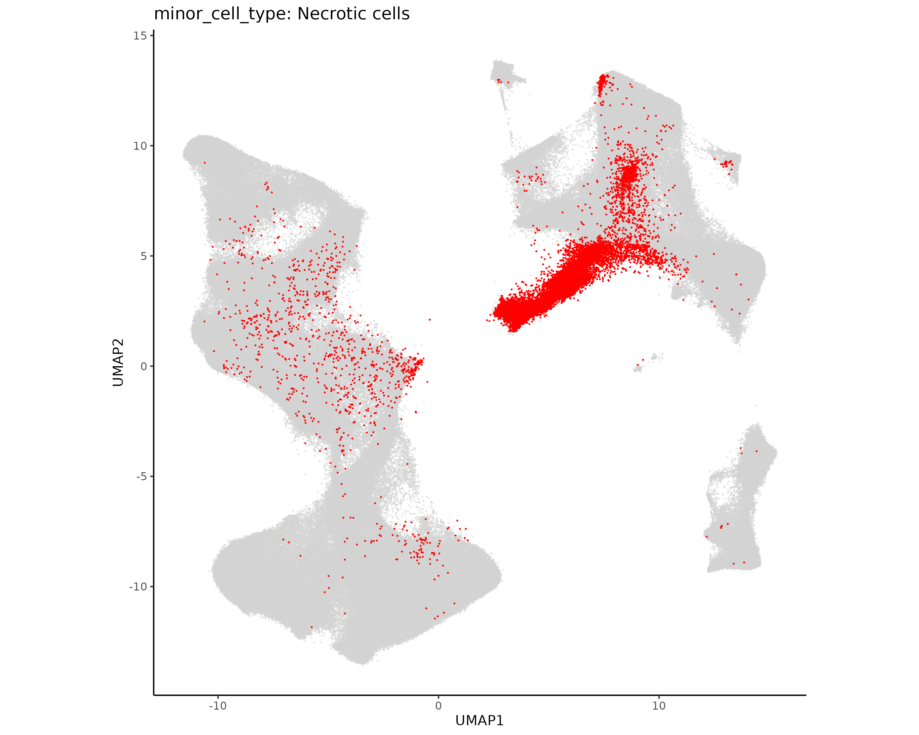
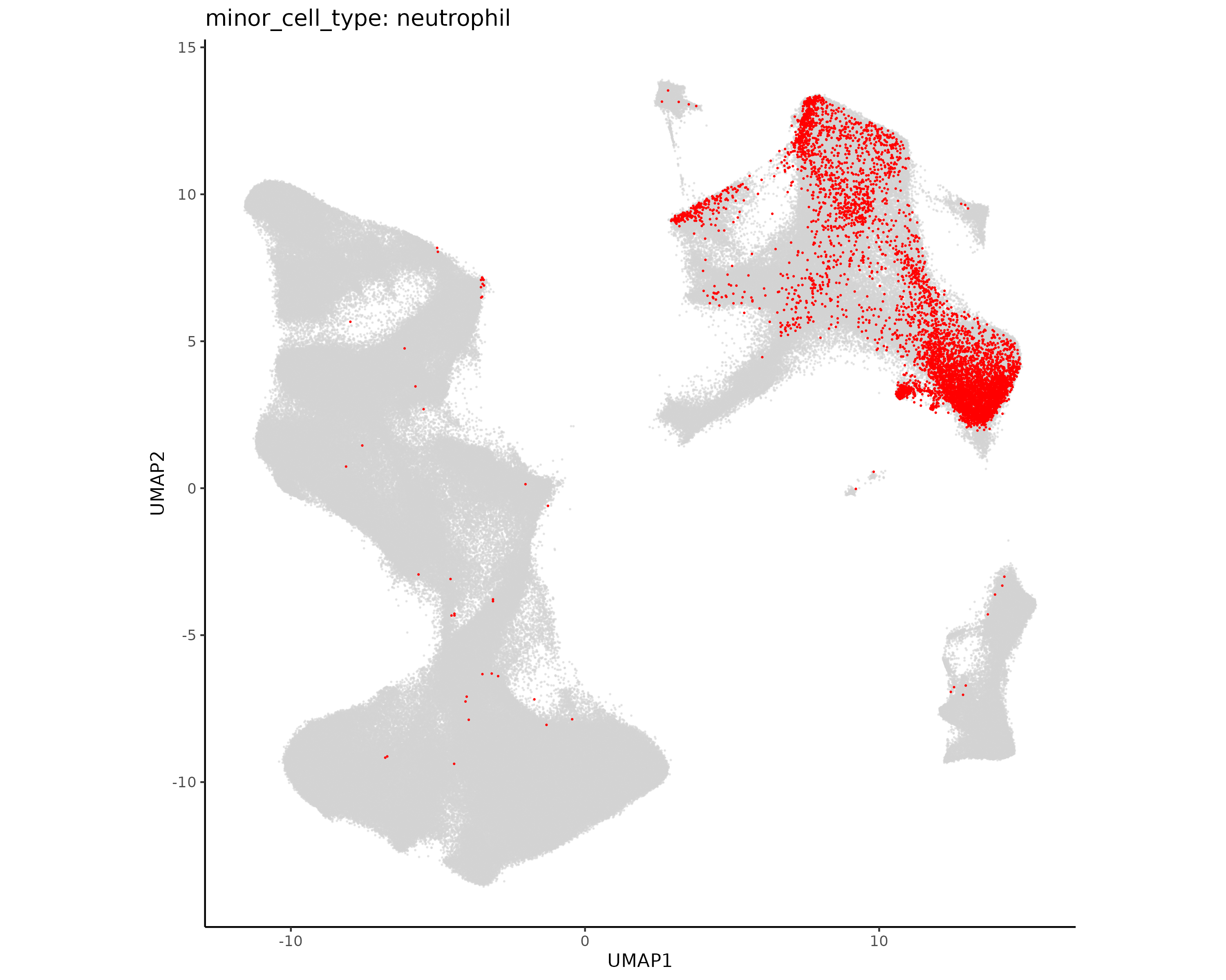
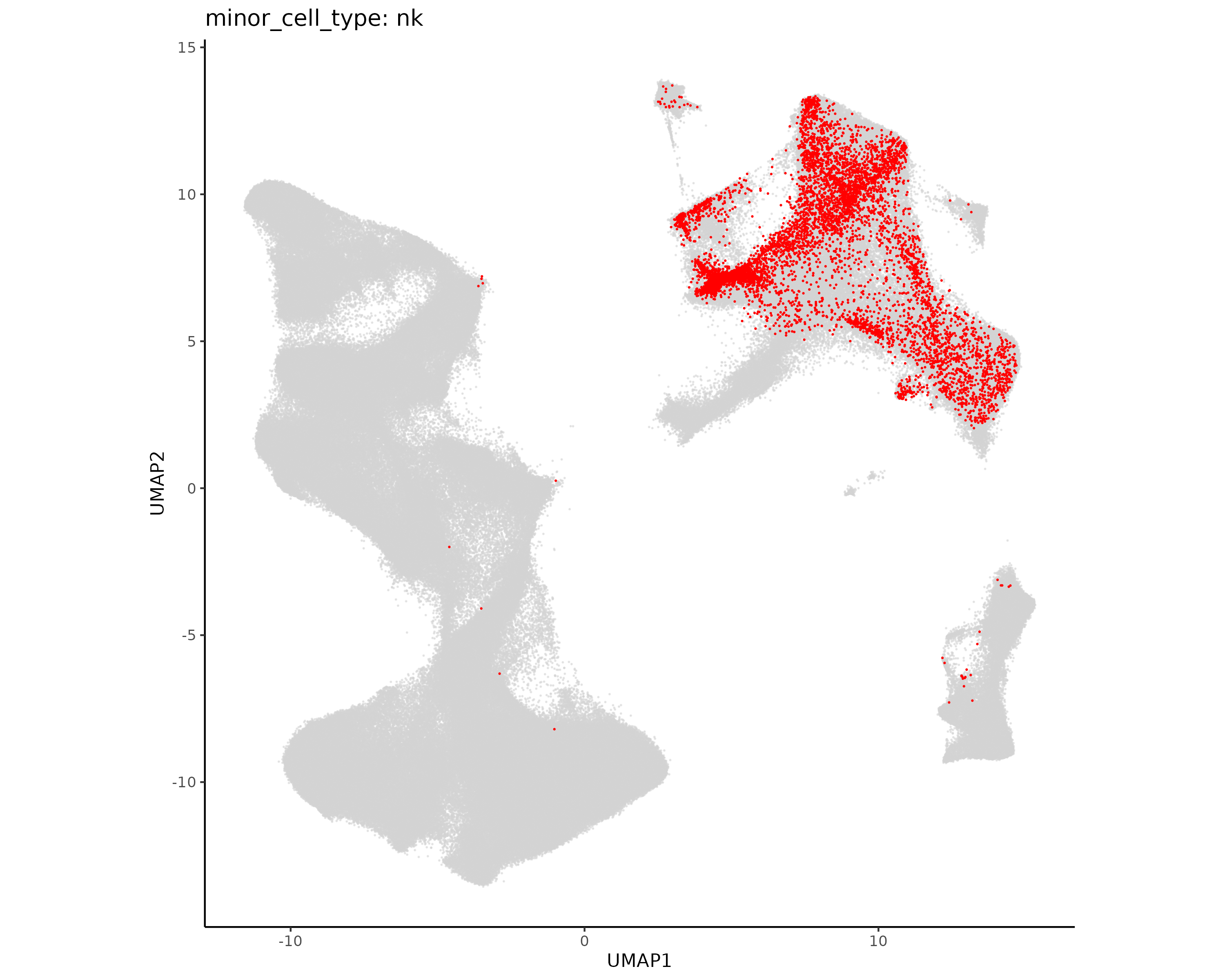
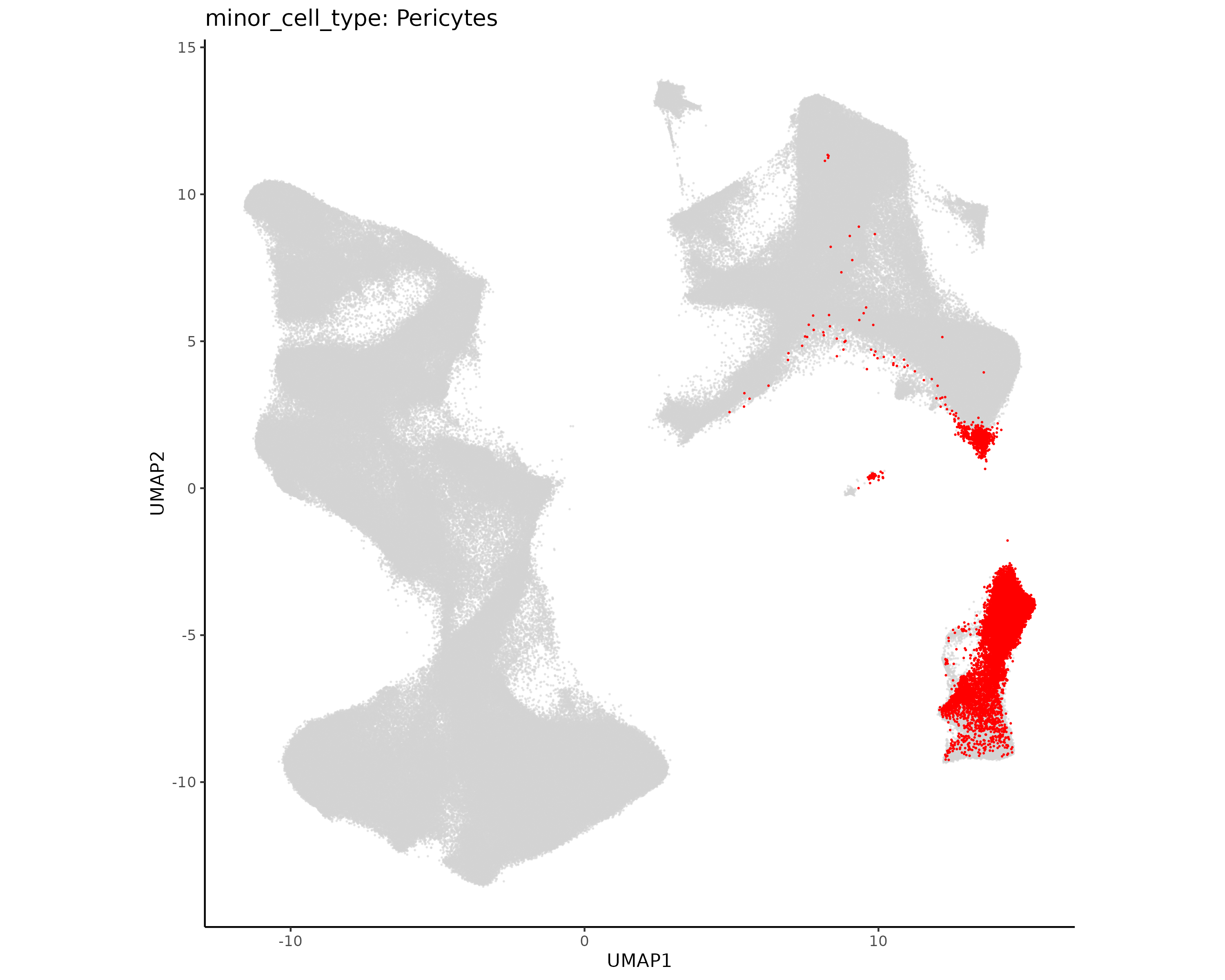
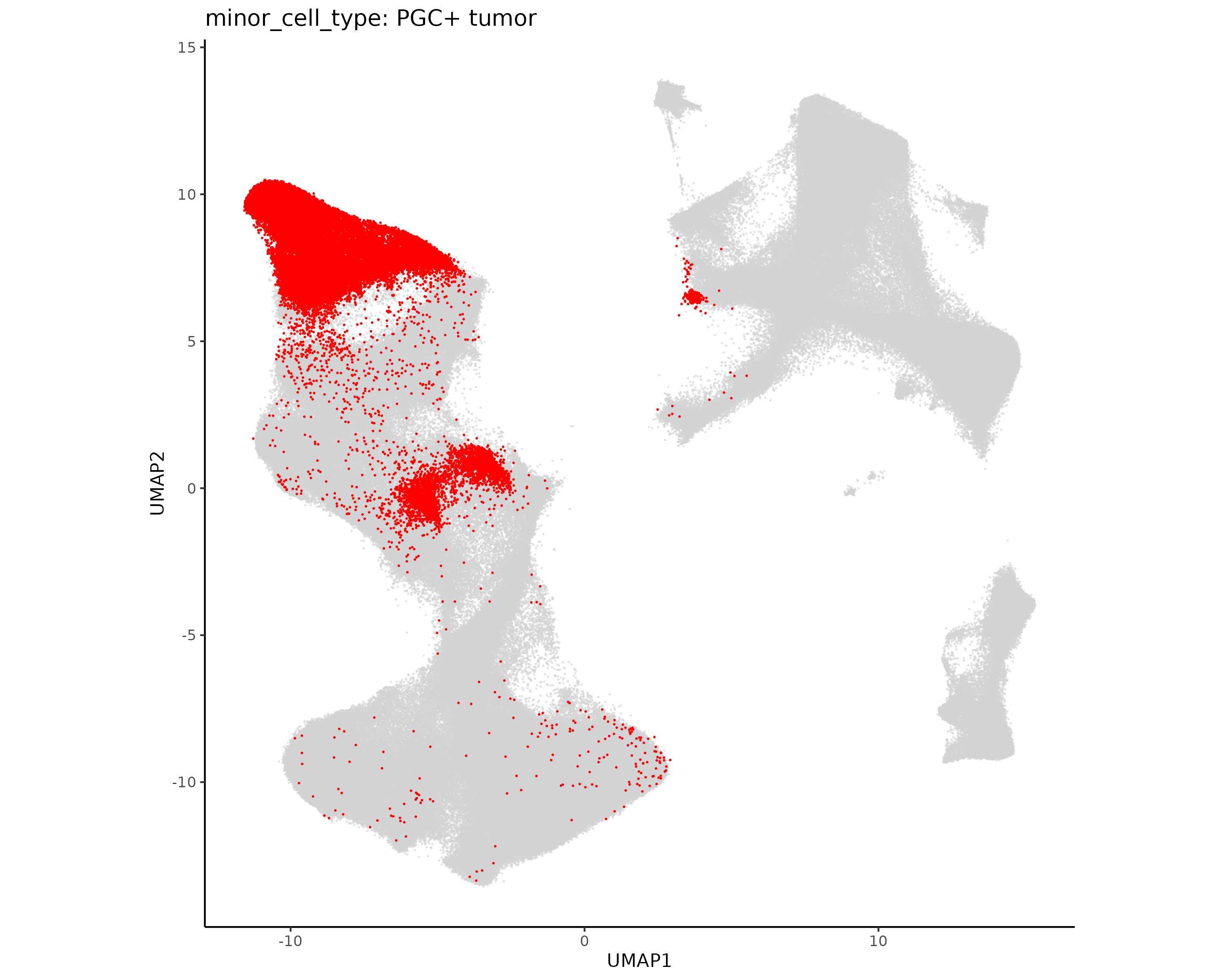
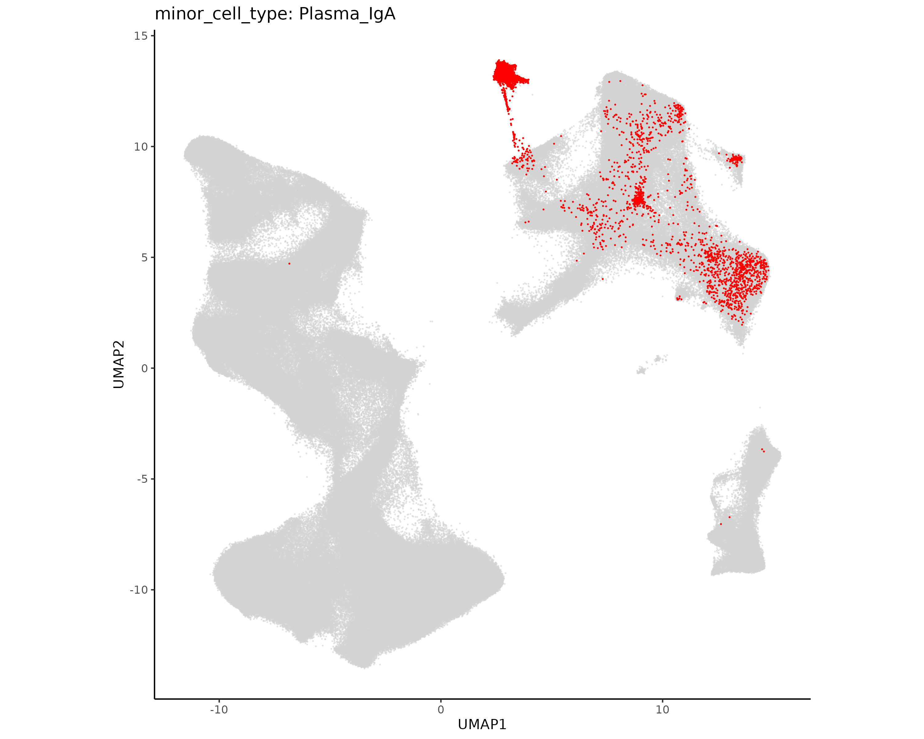
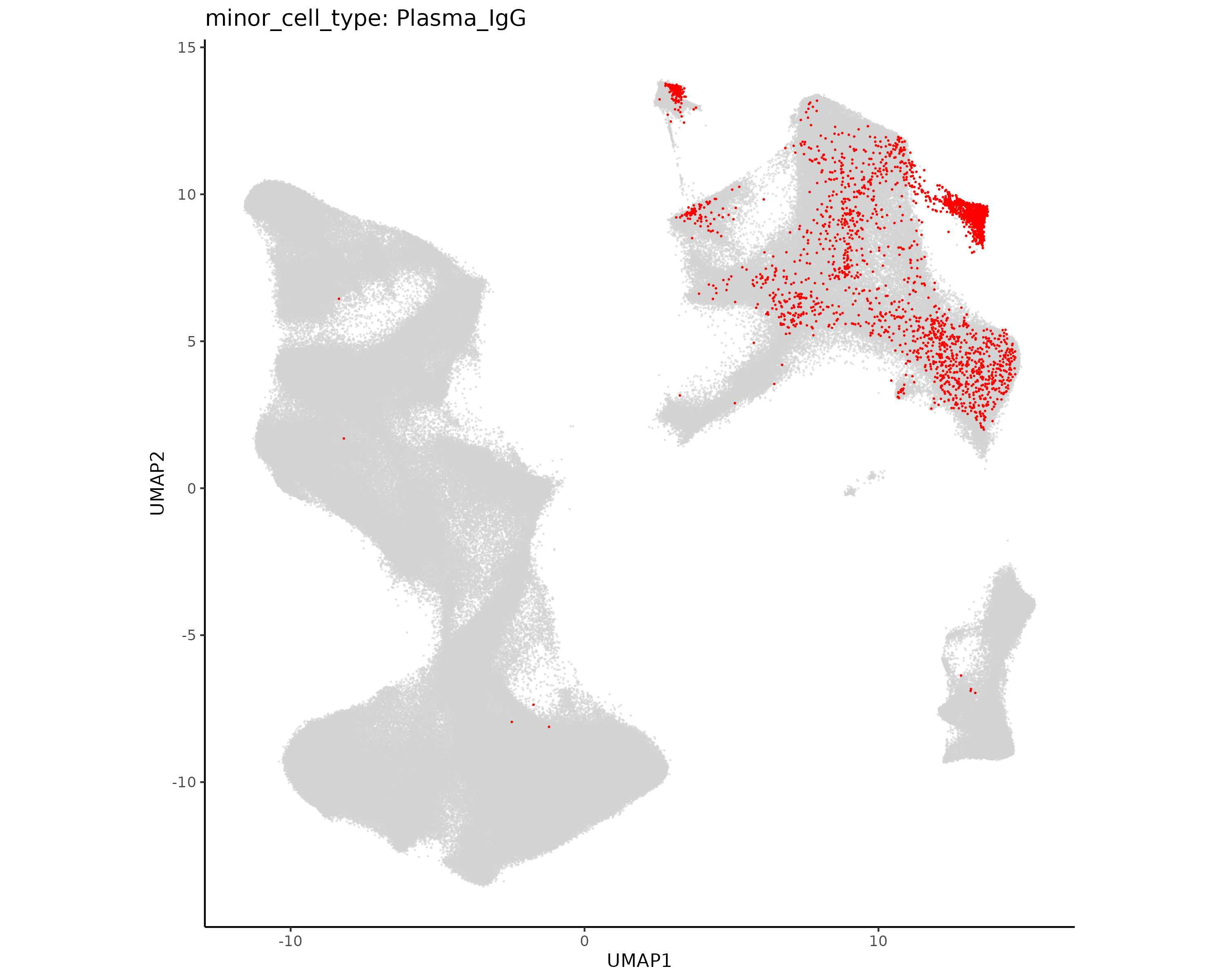
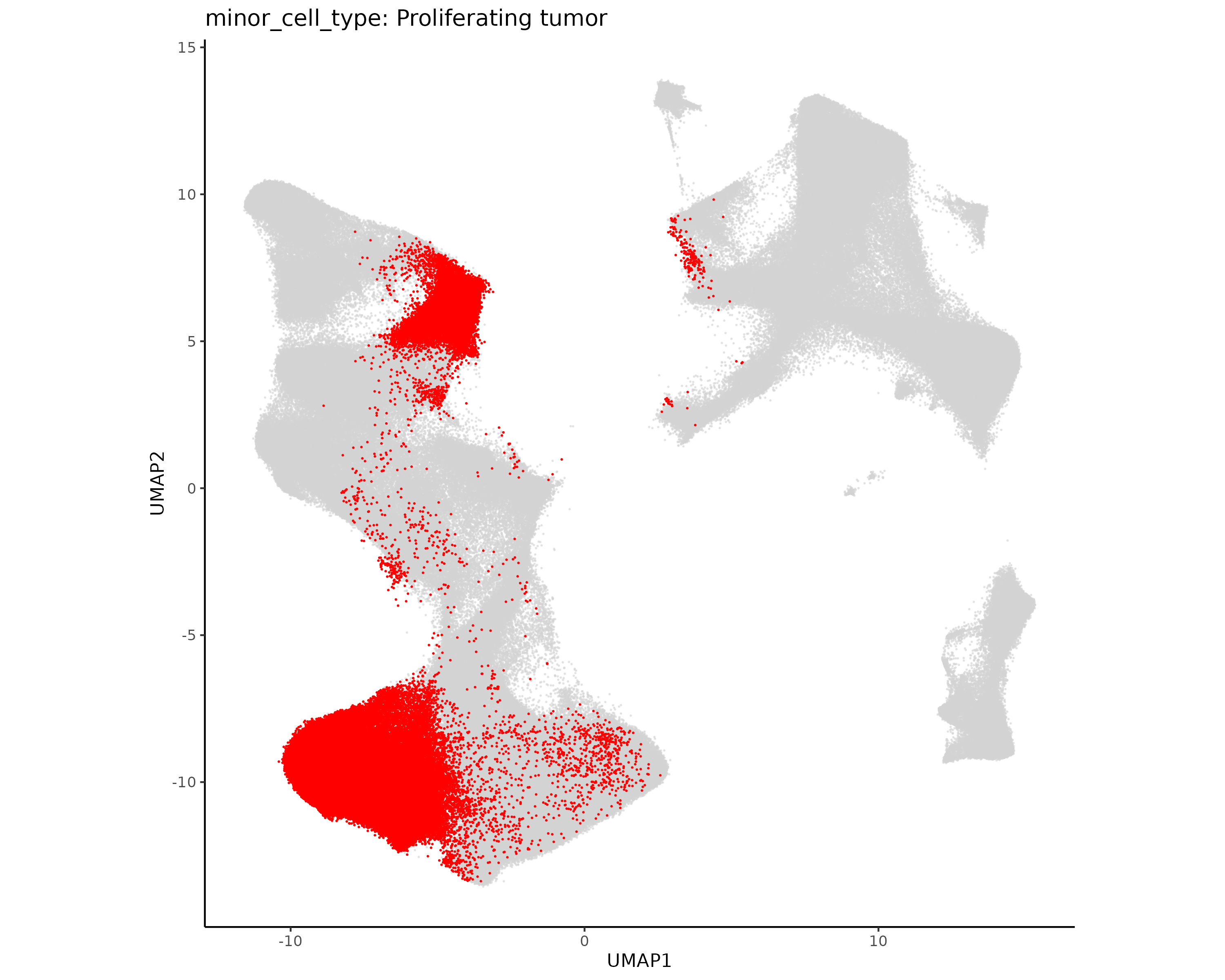
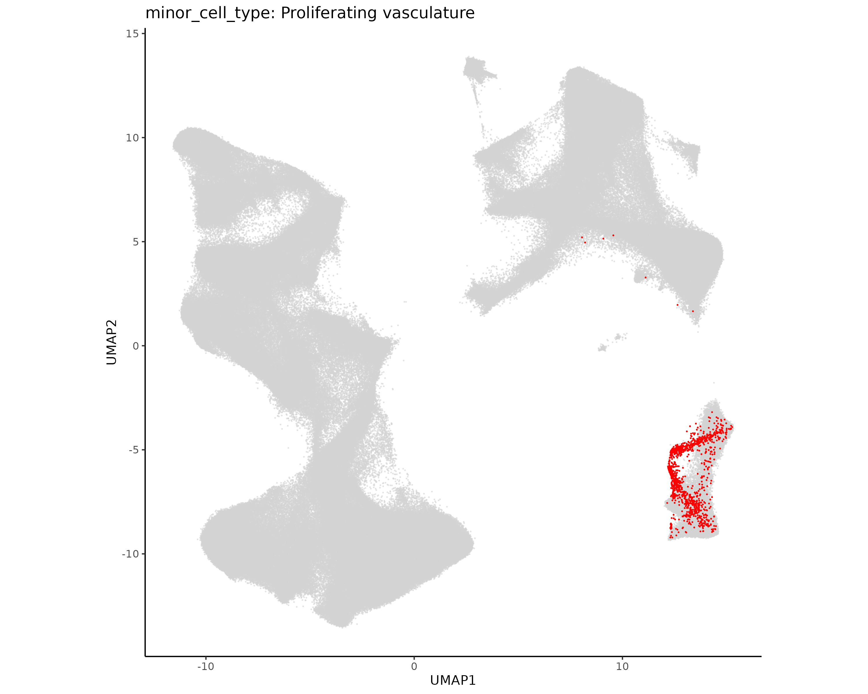
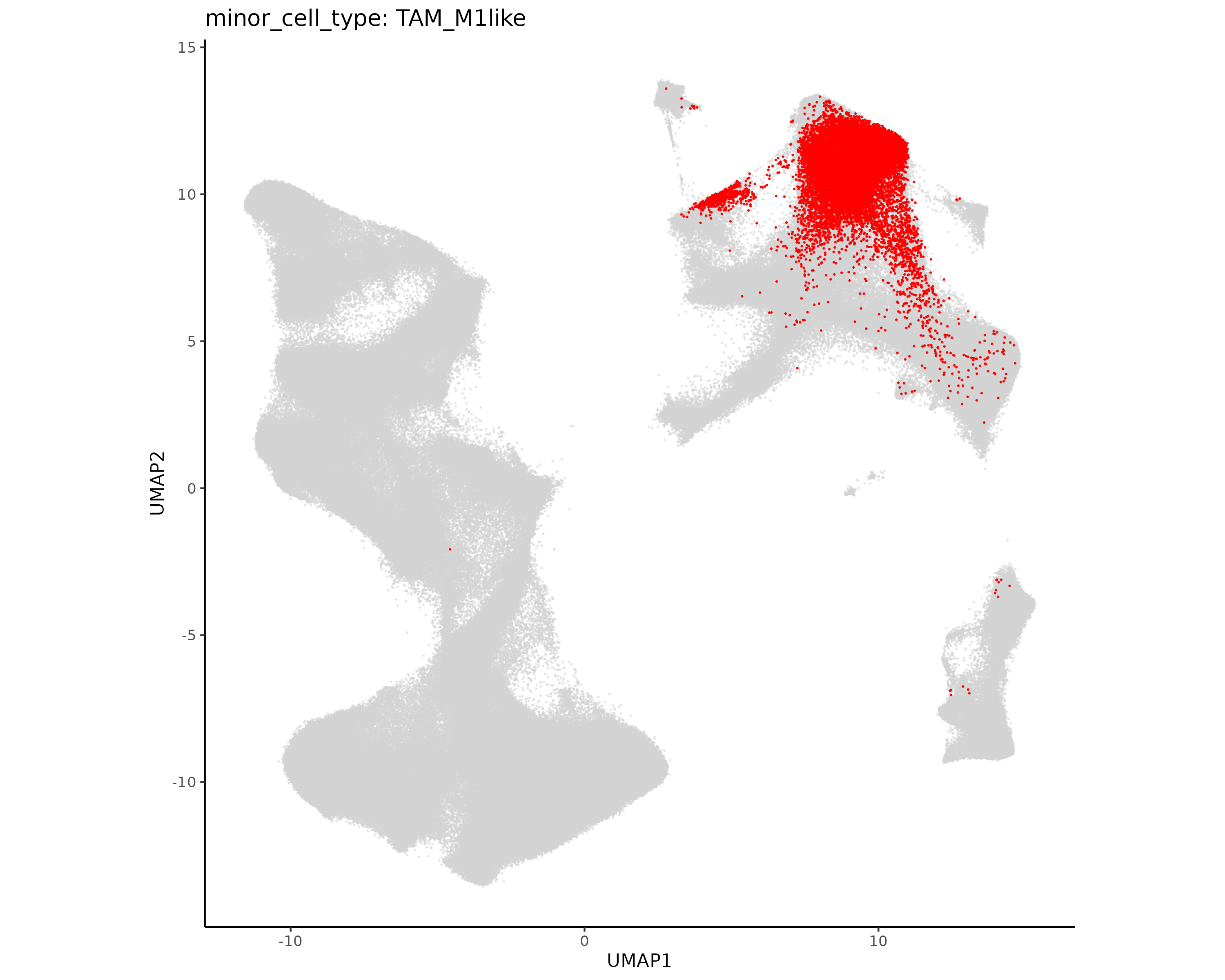
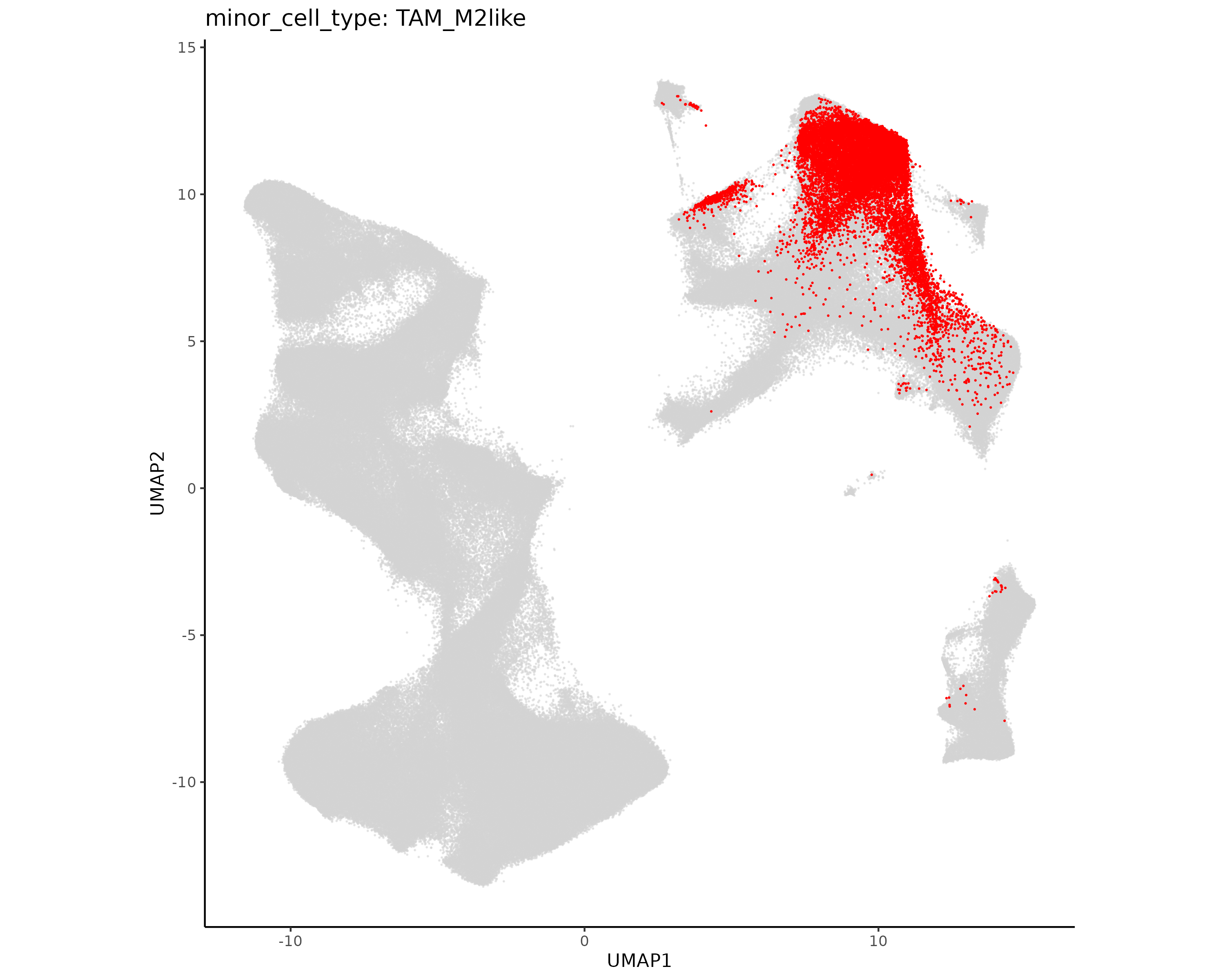
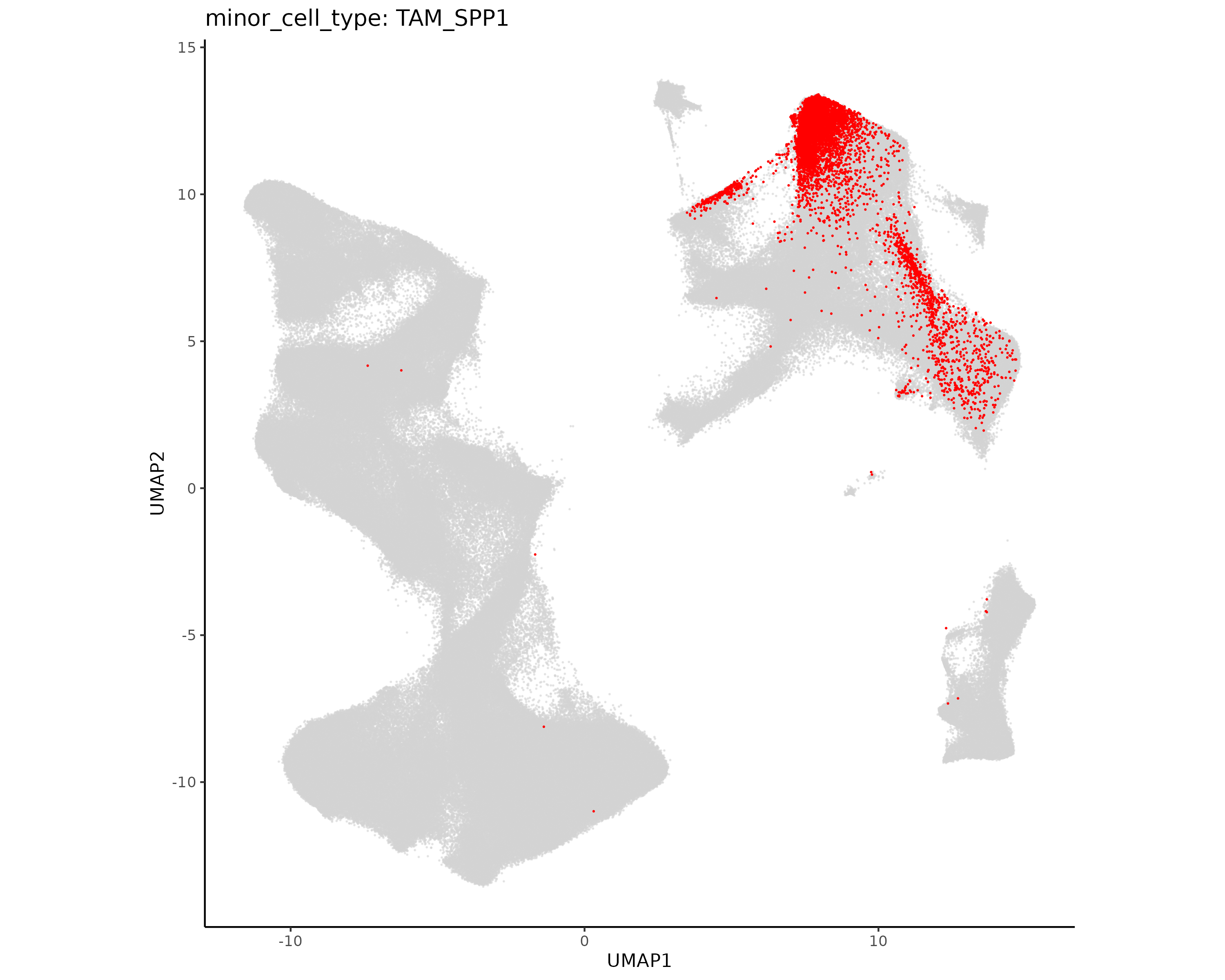
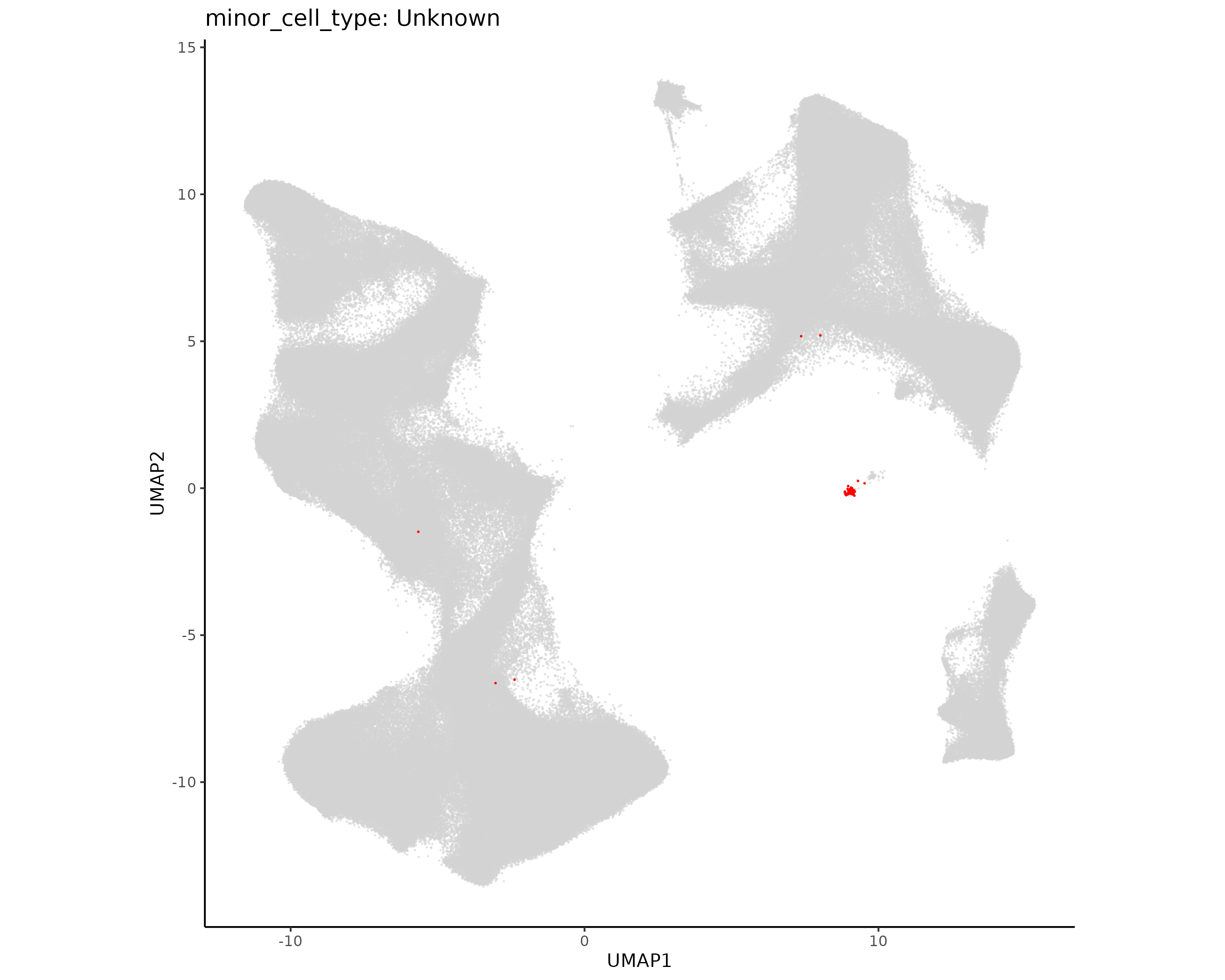
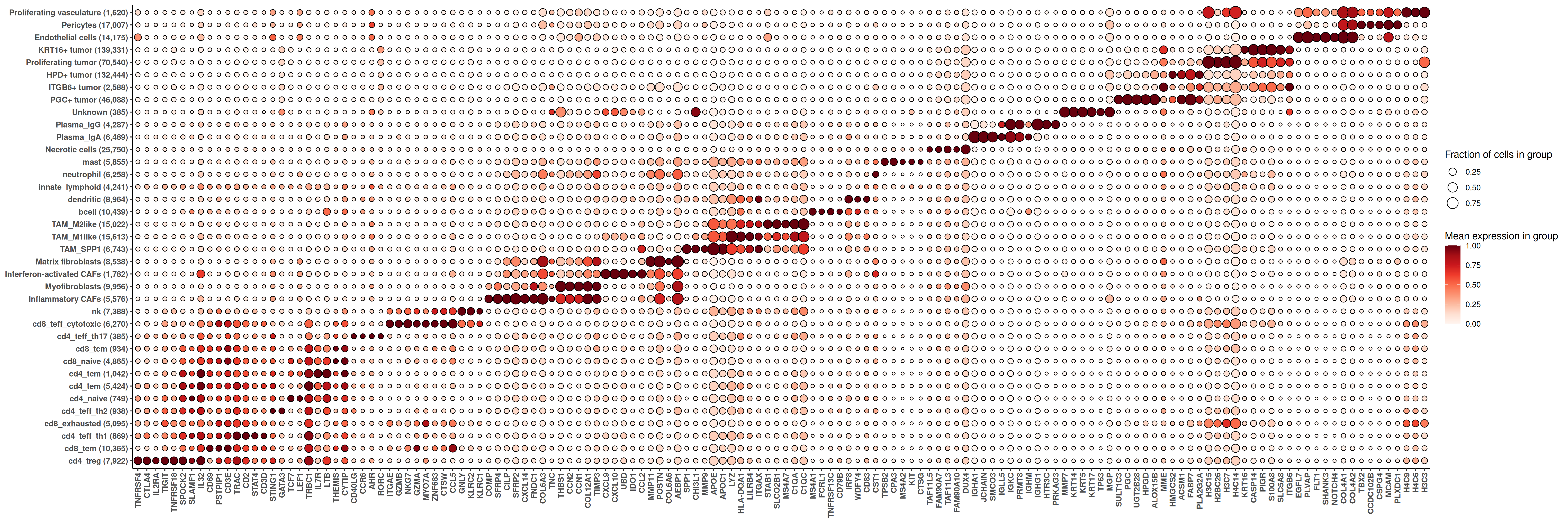
In this first chapter, we complete preprocessing steps on the breast cancer dataset. We begin with a Seurat object exported from AtoMx® SIP before any processing. We perform quality control to remove low quality cells and then proceed through normalization, dimension reduction, and cell typing.
1.1 QC
In this section we run standard QC steps on the breast cancer dataset.
Click to show/hide QC steps
1.1.1 Per Cell QC
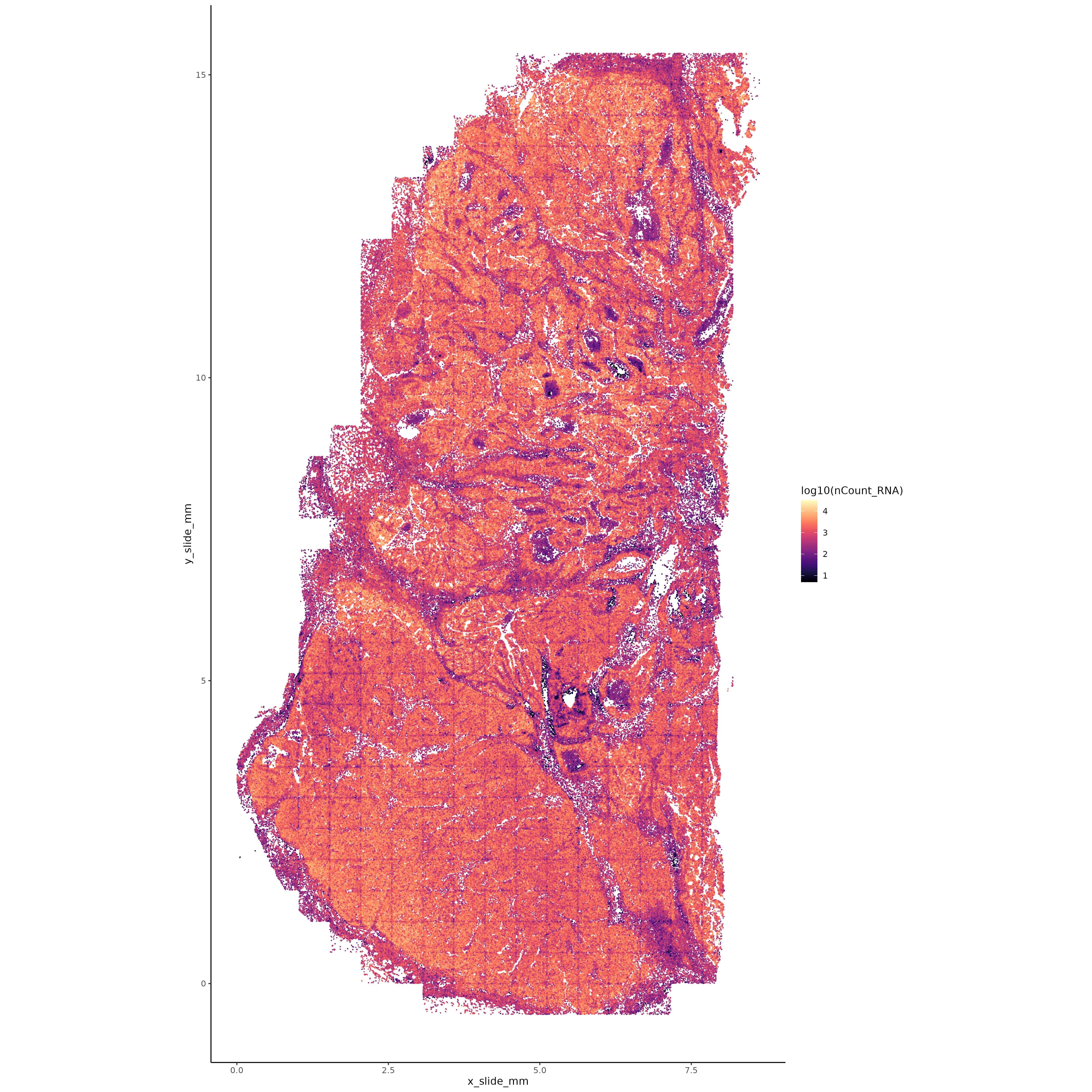
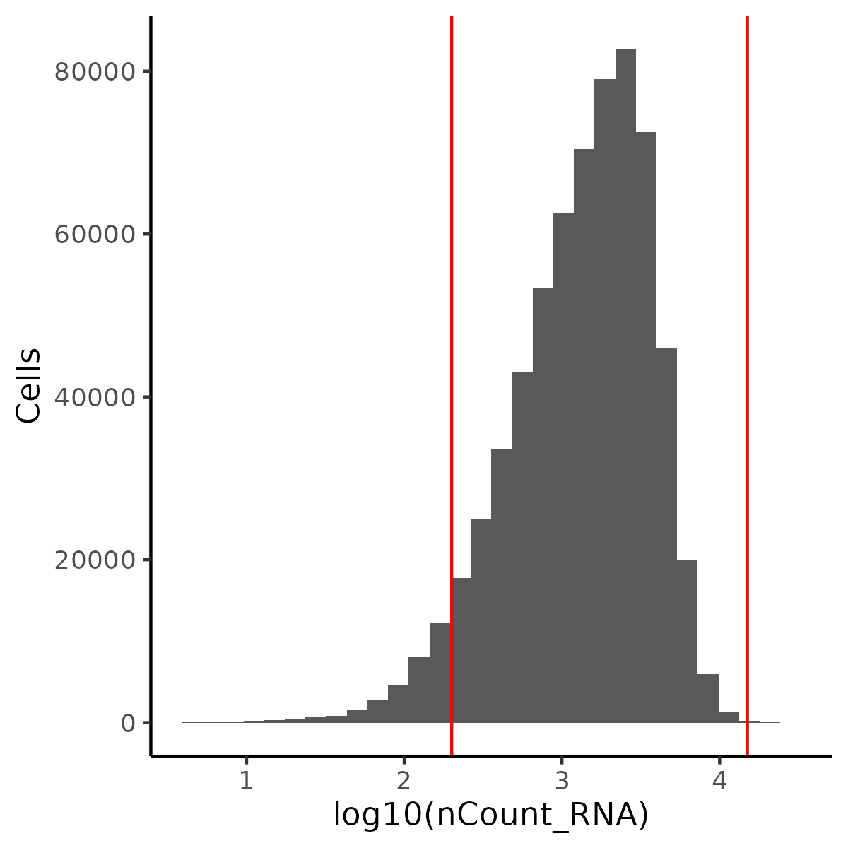
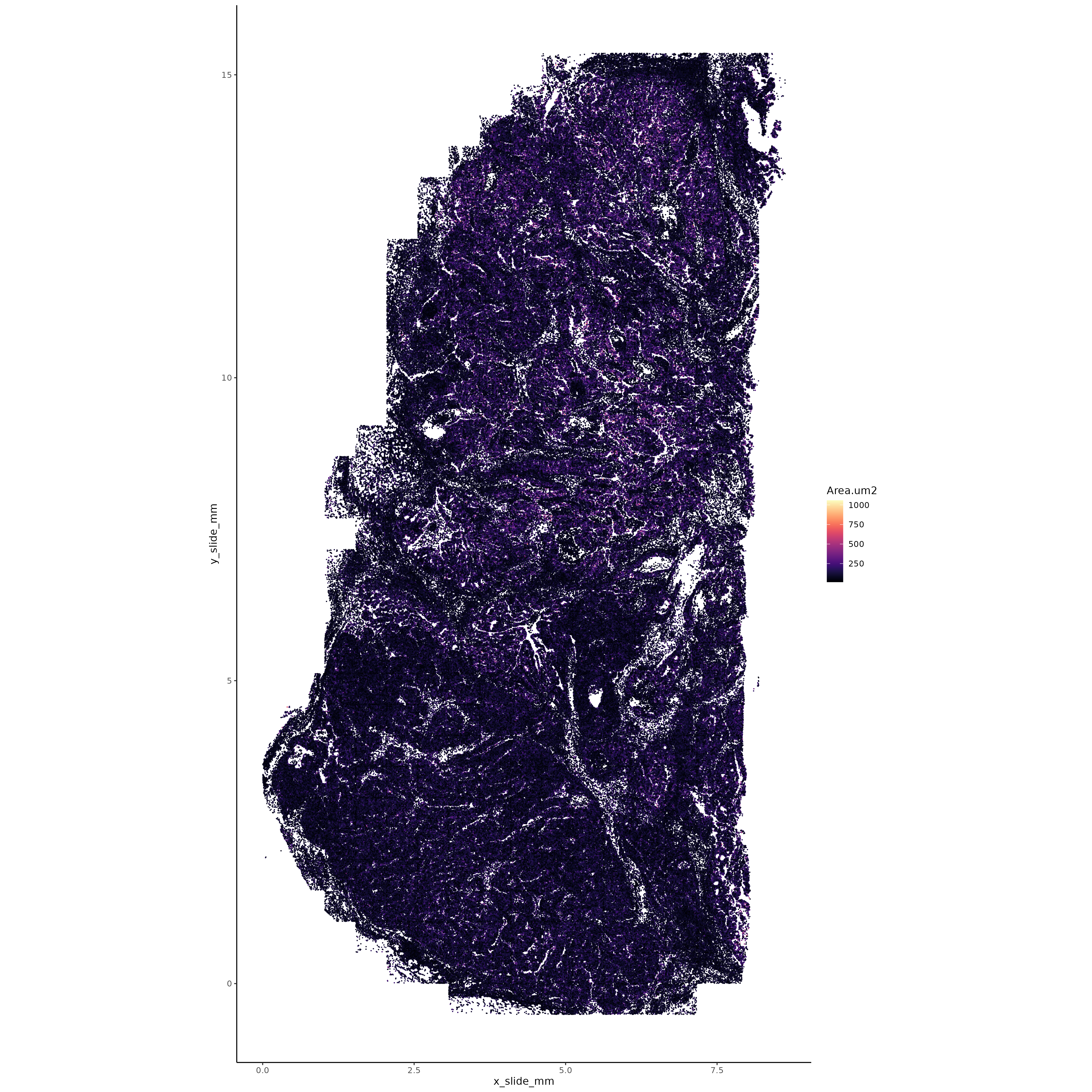
Transcripts per cell
Visualize transcripts per cell.
Show the code
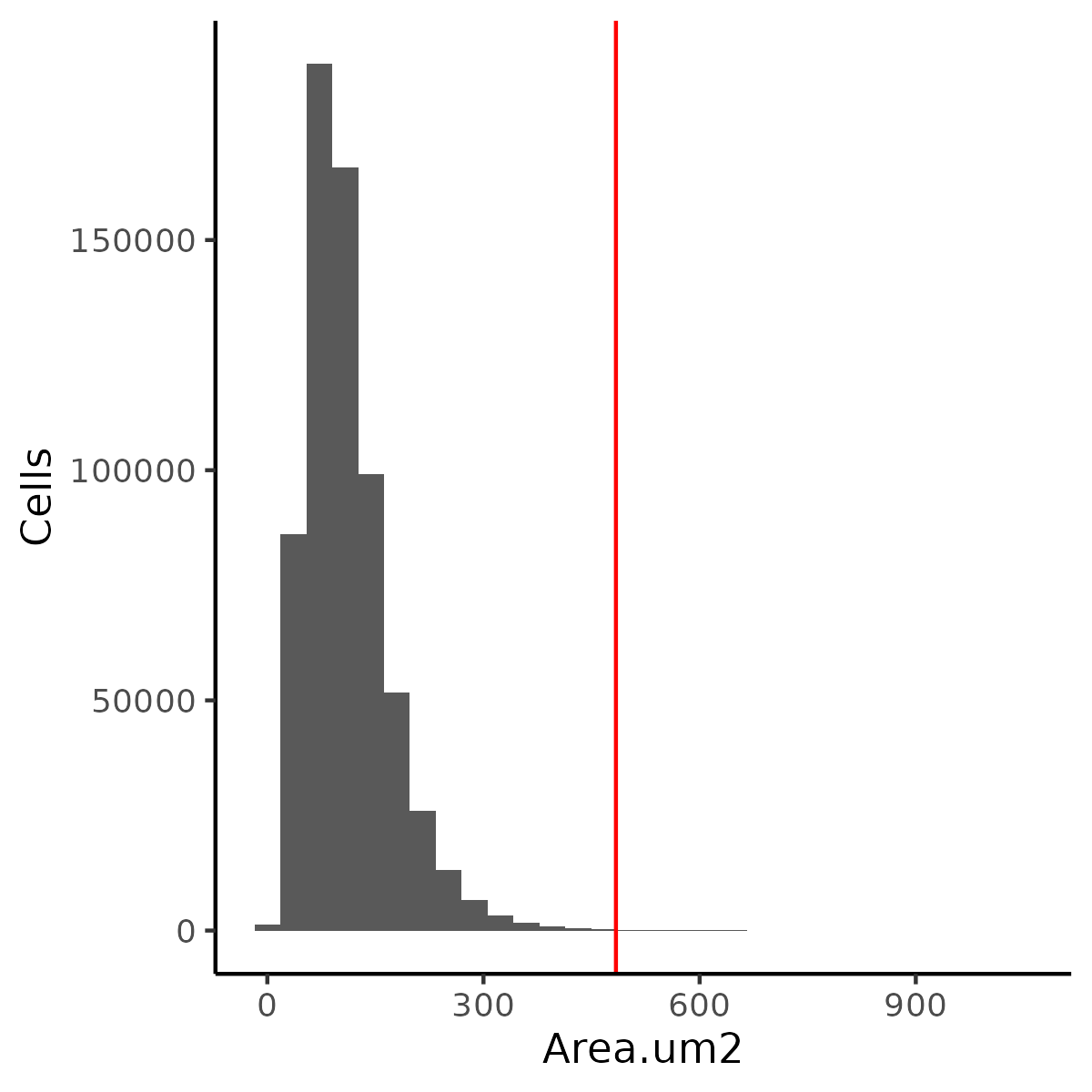
# Object and color setupif (!("seu.obj"%in%ls())){ seu.obj <-readRDS(results_list$raw_seurat_file)}# Plotting XYggplot(seu.obj@meta.data, aes(x = x_slide_mm, y = y_slide_mm, color =log10(nCount_RNA))) +geom_point(size =0.001) +scale_color_viridis(option ="A") +theme_classic() +coord_fixed() ggsave(filename =paste0(qc_dir, "/Plots/XY_txPerCell.png"),width =16, height =16, units ="in")# Plot histogram of tx per cell with cutoffslower_tx_cutoff =200# Adjust by datasetupper_tx_cutoff =15000# Adjust by datasetggplot(seu.obj@meta.data, aes(x =log10(nCount_RNA))) +geom_histogram() +geom_vline(xintercept =log10(lower_tx_cutoff), color ="red") +geom_vline(xintercept =log10(upper_tx_cutoff), color ="red") +ylab("Cells") +theme_classic()ggsave(filename =paste0(qc_dir, "/Plots/histogram_txPerCell.png"),width =4, height =4, units ="in")results_list$lower_tx_cutoff = lower_tx_cutoffresults_list$upper_tx_cutoff = upper_tx_cutoffsaveRDS(results_list, results_list_file)
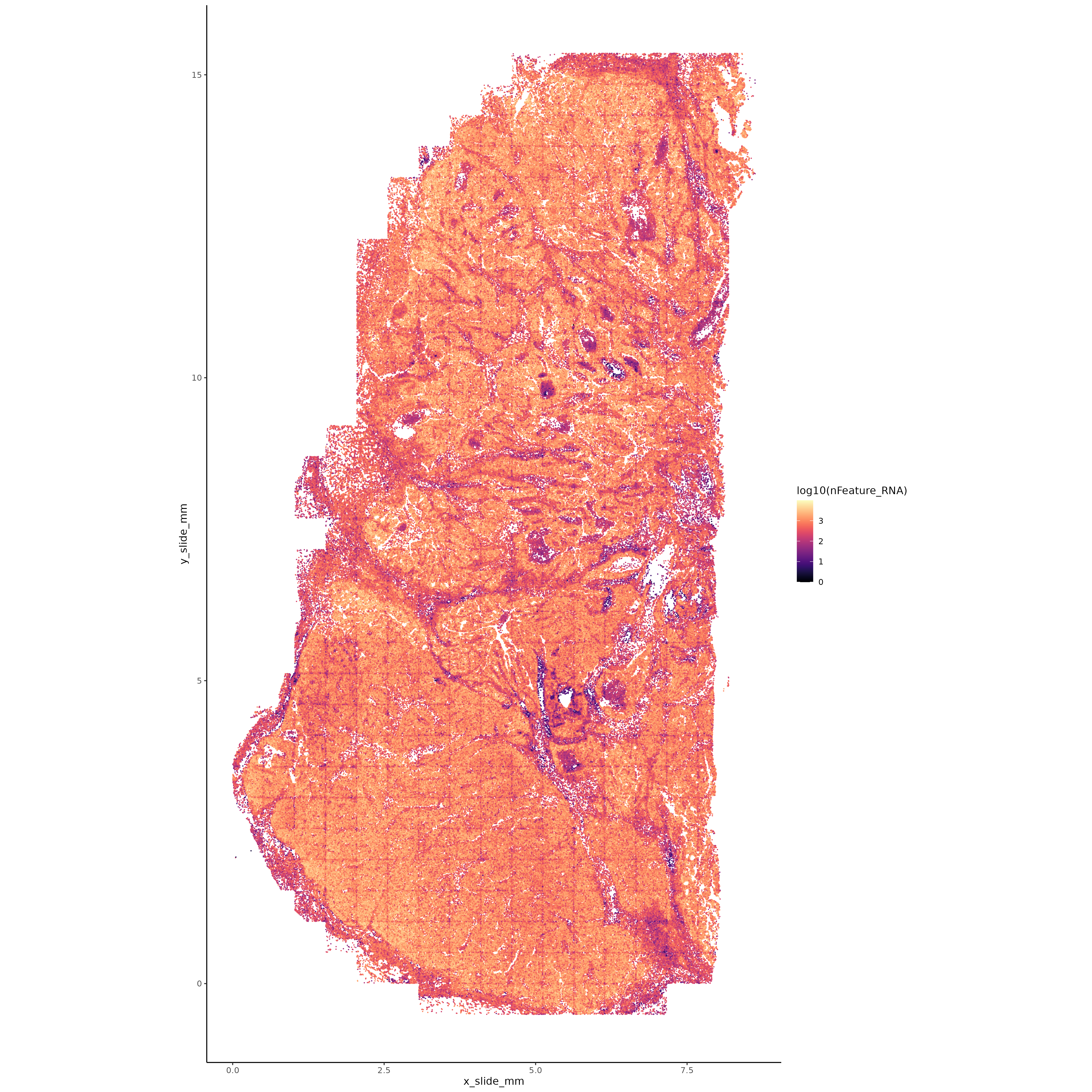
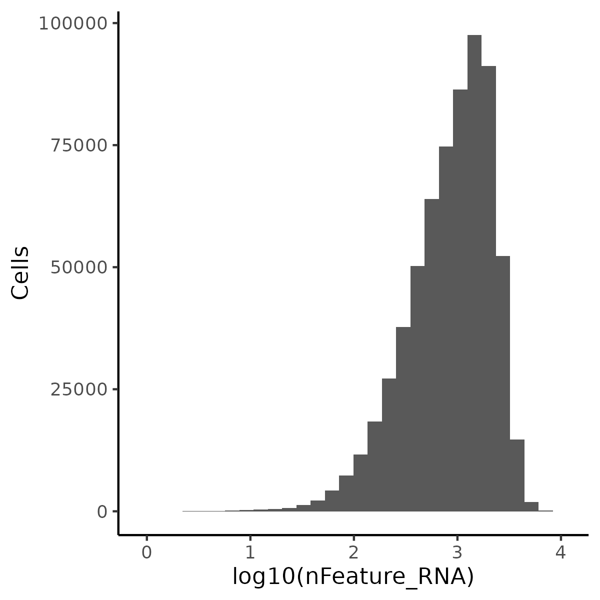
# Object and color setupif (!("seu.obj"%in%ls())){ seu.obj <-readRDS(results_list$raw_seurat_file)}# Plotting XYggplot(seu.obj@meta.data, aes(x = x_slide_mm, y = y_slide_mm, color =log10(nFeature_RNA))) +geom_point(size =0.001) +scale_color_viridis(option ="A") +theme_classic() +coord_fixed() ggsave(filename =paste0(qc_dir, "/Plots/XY_uniqueTxPerCell.png"),width =16, height =16, units ="in")# Plot histogram of tx per cell with no cutoffs shown (non-standard to use them)ggplot(seu.obj@meta.data, aes(x =log10(nFeature_RNA))) +geom_histogram() +ylab("Cells") +theme_classic()ggsave(filename =paste0(qc_dir, "/Plots/histogram_uniqueTxPerCell.png"),width =4, height =4, units ="in")
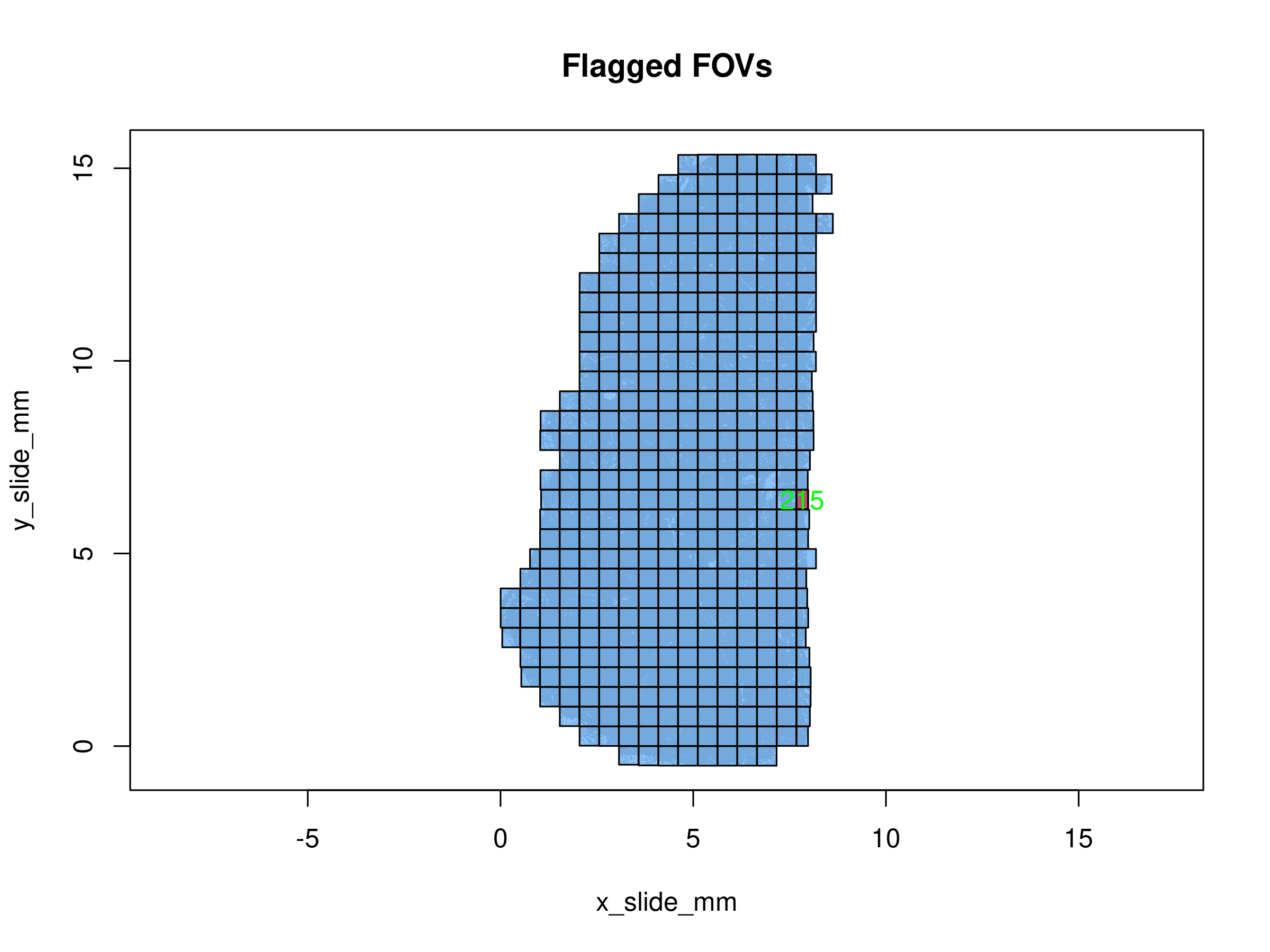
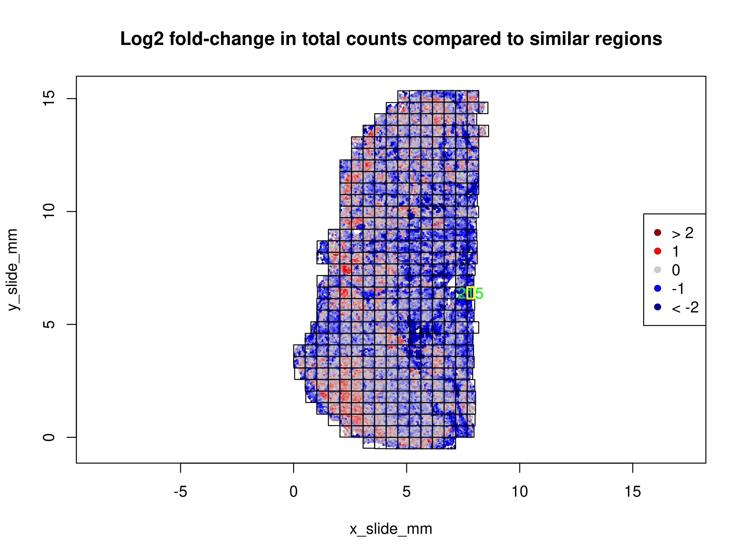
There is one FOV that gets flagged due to low counts. As this is on the edge of the tissue, this is not too surprising and we will keep this FOV in our analysis.
The changes in total signal strength tend to follow biology and do not track with individual FOVs. Thus, we will not exclude any FOVs for further analysis based on these results.
1.1.3 Cell Flagging
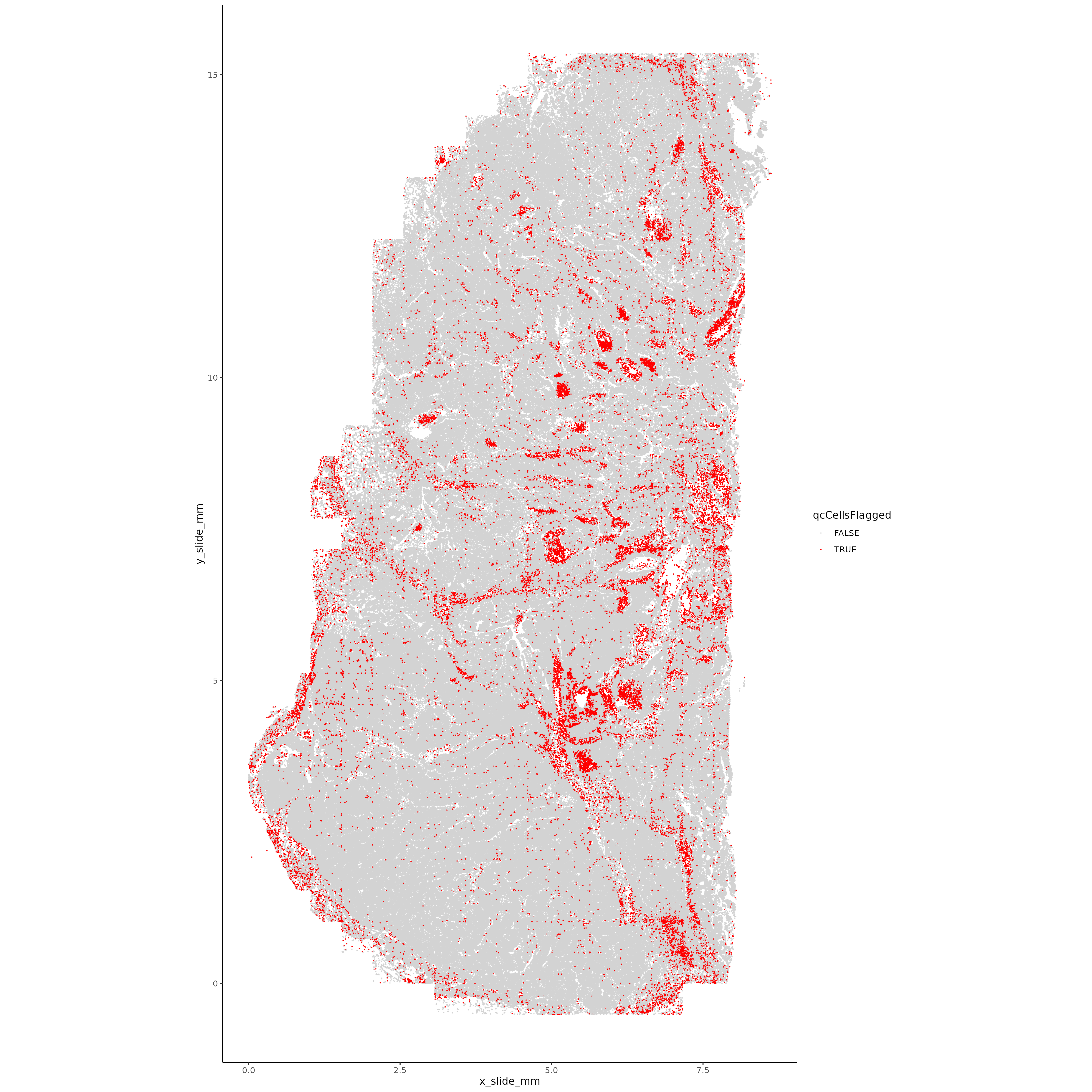
Flag cells that failed any of the QC above and plot these in space. We’re looking for areas with high failure rates, suggesting technical artifacts (local tissue peeling, blurriness, etc).
Show the code
# Object and color setupif (!("seu.obj"%in%ls())){ seu.obj <-readRDS(results_list$raw_seurat_file)}# Flag cells that failed tx or area QCseu.obj@meta.data <- seu.obj@meta.data %>%mutate(qcCellsFlagged =case_when( Area.um2 > area_cutoff ~"TRUE", nCount_RNA < lower_tx_cutoff ~"TRUE", nCount_RNA > upper_tx_cutoff ~"TRUE",TRUE~"FALSE" ))# Plotting XYggplot(seu.obj@meta.data, aes(x = x_slide_mm, y = y_slide_mm, color = qcCellsFlagged)) +geom_point(size =0.001) +scale_color_manual(values =c("FALSE"="lightgrey", "TRUE"="red")) +theme_classic() +coord_fixed() ggsave(filename =paste0(qc_dir, "/Plots/XY_QCflaggedCells.png"),width =16, height =16, units ="in")# Remove cells failing QC and save seurat objectseu.obj <- seu.obj[,which(seu.obj@meta.data$qcCellsFlagged =="FALSE")]saveRDS(seu.obj, file =paste0(objects_dir, "/seurat_object_postQC.rds"))results_list$seurat_file_postQC =paste0(objects_dir, "/seurat_object_postQC.rds")saveRDS(results_list, results_list_file)
From this plot, it’s clear that the flagged cells aren’t evenly spread across the tissue - there are round-ish structures that are getting flagged at a much higher rate, suggesting that there’s a structure in the tissue that has lower counts for some reason. Given this, we have used a liberal cutoff of 200 counts per cell. From a bit of exploration, it’s clear that these cells are primarily getting flagged due to having low counts. Returning to the immunofluorescence images, these likely mark regions of necrosis.
1.2 Normalization
In this section we run basic normalization on the data.
Click to show/hide normalization steps
1.2.1 Total counts normalization
Run total counts normalization with Seurat function.
Show the code
# Object and color setupif (!("seu.obj"%in%ls())){ seu.obj <-readRDS(results_list$seurat_file_postQC)}# With Seuratseu.obj <-NormalizeData(seu.obj, normalization.method ="RC", scale.factor =mean(seu.obj@meta.data$nCount_RNA))
1.2.2 Highly variable genes
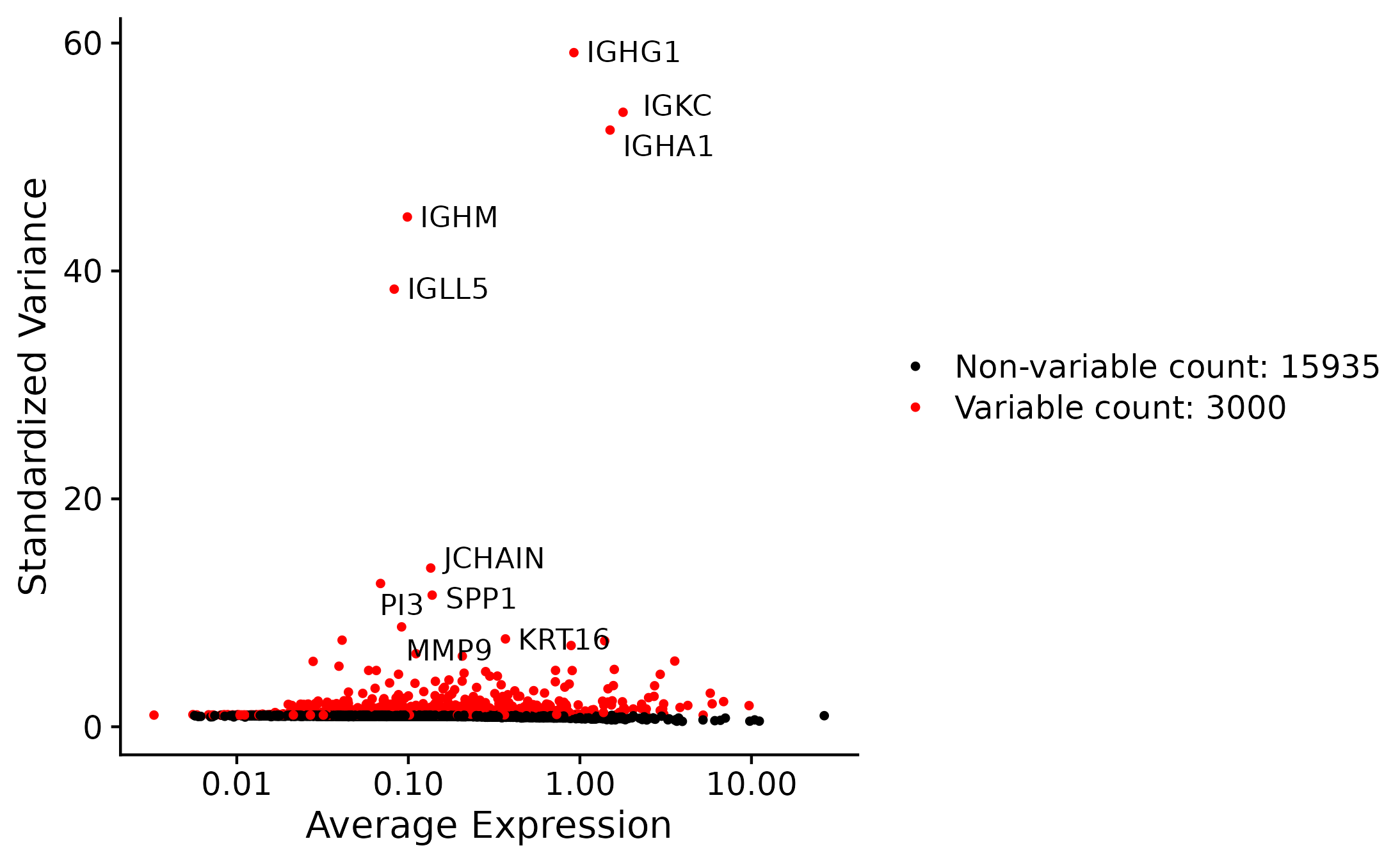
Identify highly variable genes
Show the code
# With Seuratseu.obj <-FindVariableFeatures(seu.obj, selection.method ="vst", nfeatures =3000)# Get top 10 variable features to labeltop10 <-head(VariableFeatures(seu.obj), 10)# plot variable features with and without labelsplot1 <-VariableFeaturePlot(seu.obj)plot2 <-LabelPoints(plot = plot1, points = top10, repel =TRUE)plot2ggsave(plot = plot2, filename =paste0(norm_dir, "/Plots/hvgs.png"))# Save HVGs to a vectorsaveRDS(VariableFeatures(seu.obj), file =paste0(norm_dir, "/Data/hvgs.rds"))# Save Seurat object post-normalization and HVG identificationsaveRDS(seu.obj, file =paste0(objects_dir, "/seurat_object_postNorm.rds"))results_list$seurat_file_postNorm =paste0(objects_dir, "/seurat_object_postNorm.rds")saveRDS(results_list, results_list_file)
Plot of the most variable genes - largely IgGs and some cancer-related genes.
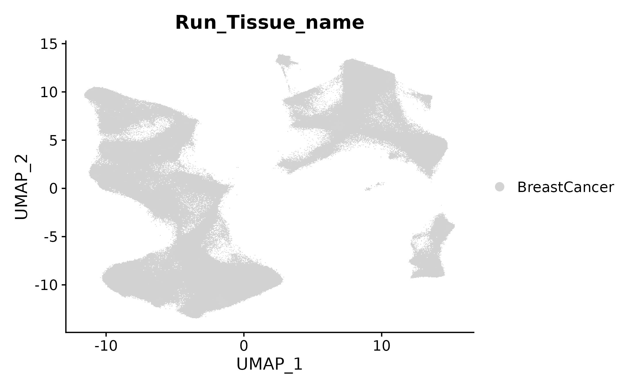
Run UMAP with the uwot package and then add that to the Seurat object.
Show the code
# Make umap with a function using uwot packageumapobj <-make_umap(seu.obj@reductions$pca@cell.embeddings)seu.obj[["umap"]] <- umapobj$umpseu.obj[["umapgrph"]] <- Seurat::as.Graph(umapobj$grph)# Plot itDimPlot(seu.obj, reduction ="umap", cols ="lightgrey", group.by ="Run_Tissue_name")ggsave(filename =paste0(dimRed_dir, "/Plots/umap.png"))# Save the seurat object with these initial stepssaveRDS(seu.obj, file =paste0(objects_dir, "/seurat_object_postUMAP.rds"))results_list$seurat_file_postUMAP =paste0(objects_dir, "/seurat_object_postUMAP.rds")saveRDS(results_list, results_list_file)
In this section we assign major and minor cell types using a combination of iterative unsupervised clustering and marker-based hierarchical assignment.
Click to show/hide cell typing steps
This section performs cell typing of the dataset with a multistep approach. First, we use unsupervised clustering to broadly group the cells. For some of these major cell types (tumor cells, fibroblasts, vascular cells) we subset and perform unsupervised clustering a second time on the subset. For immune cells, we use the marker-based hierarchical cell typing approach HieraType.
1.4.1 Unsupervised clustering
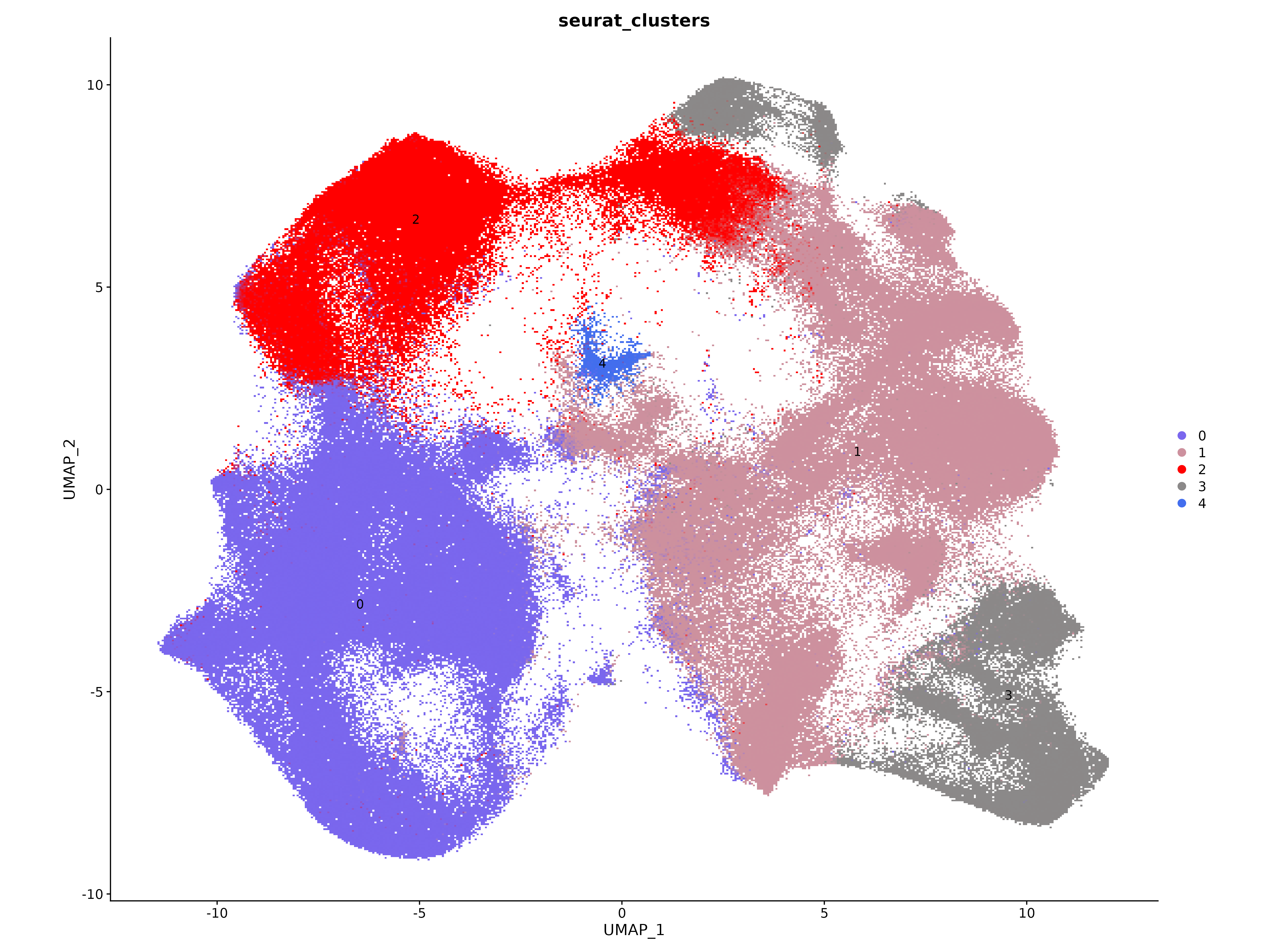
Cluster cells with Seurat function.
Show the code
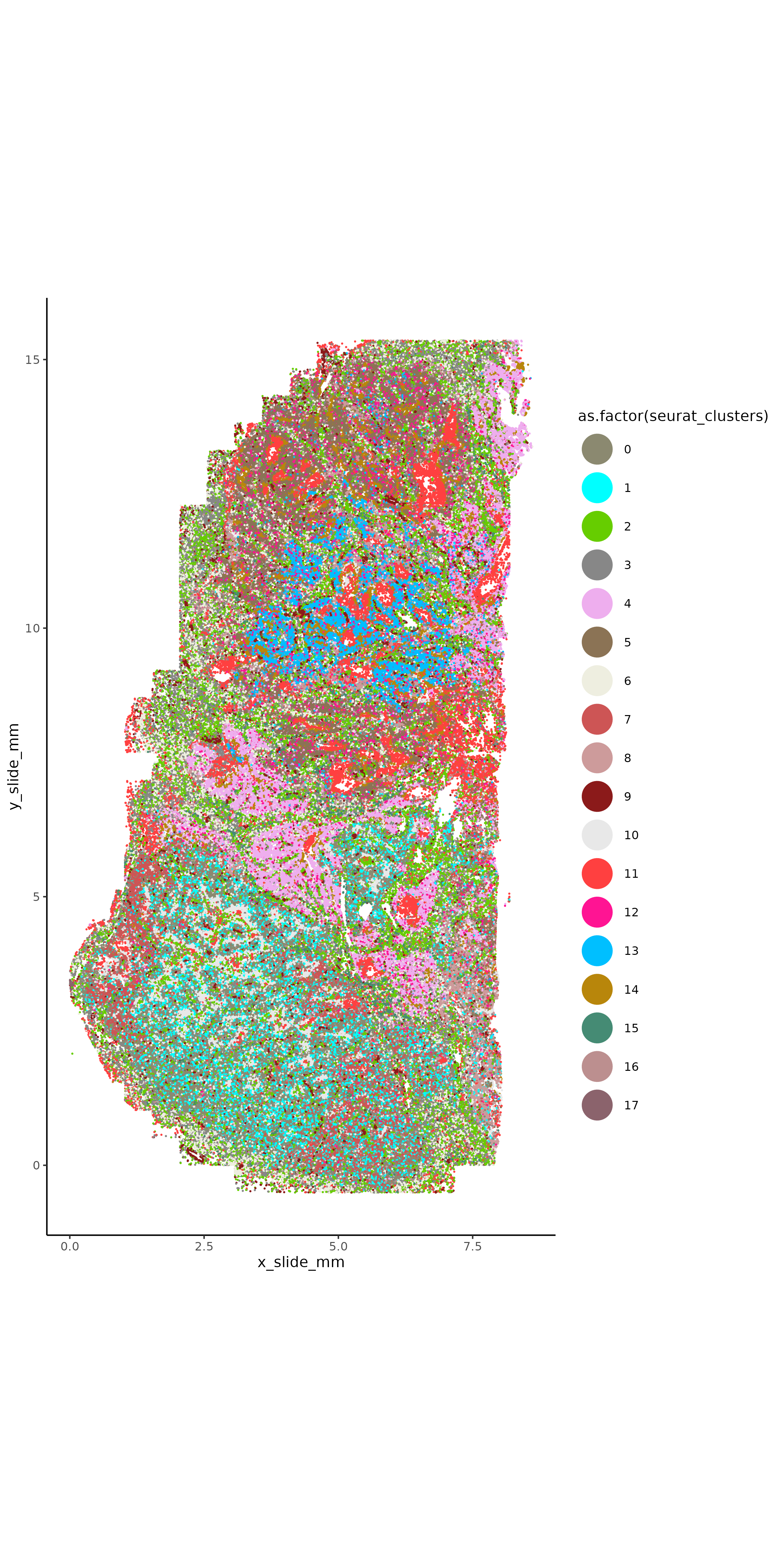
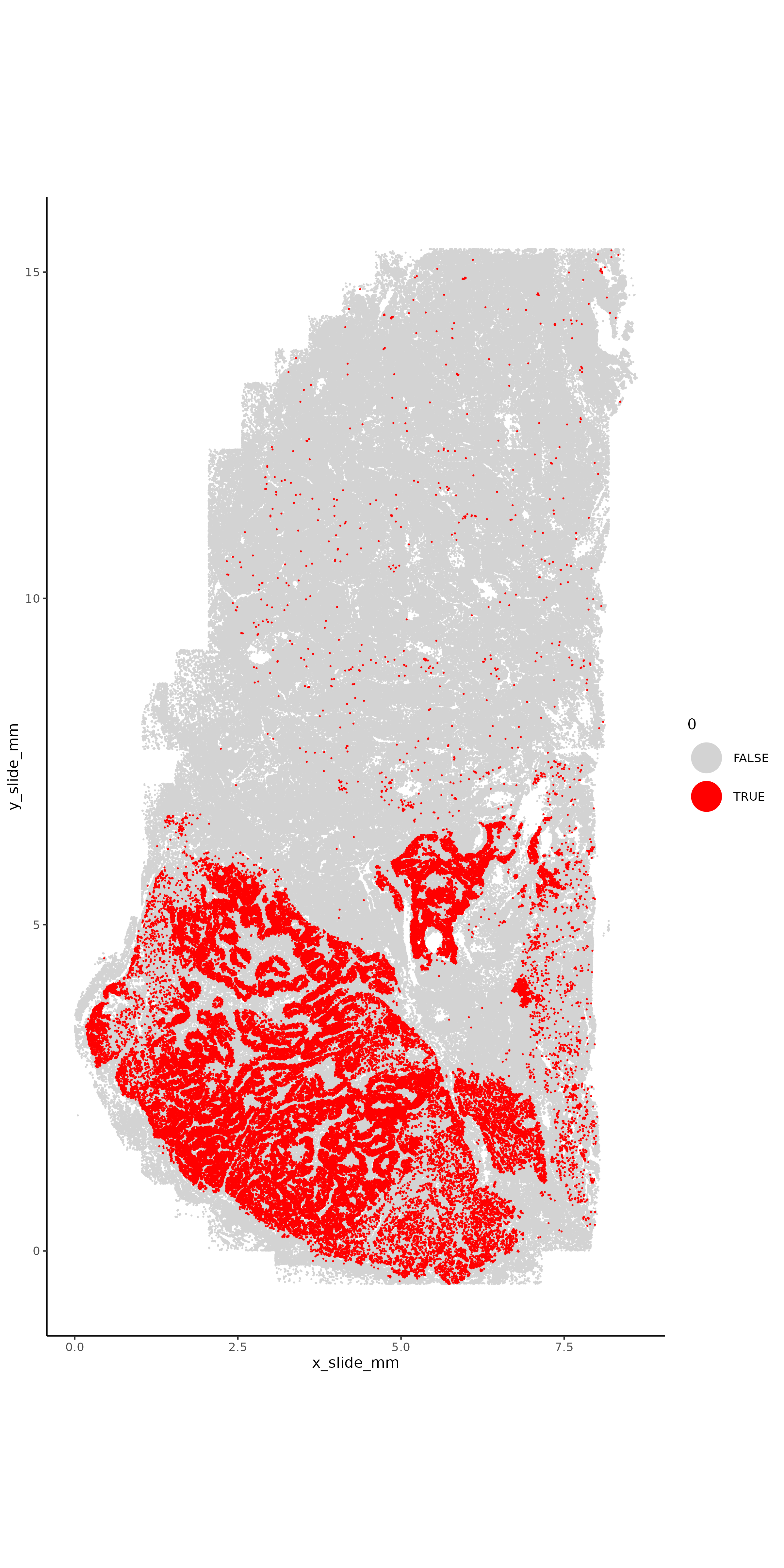
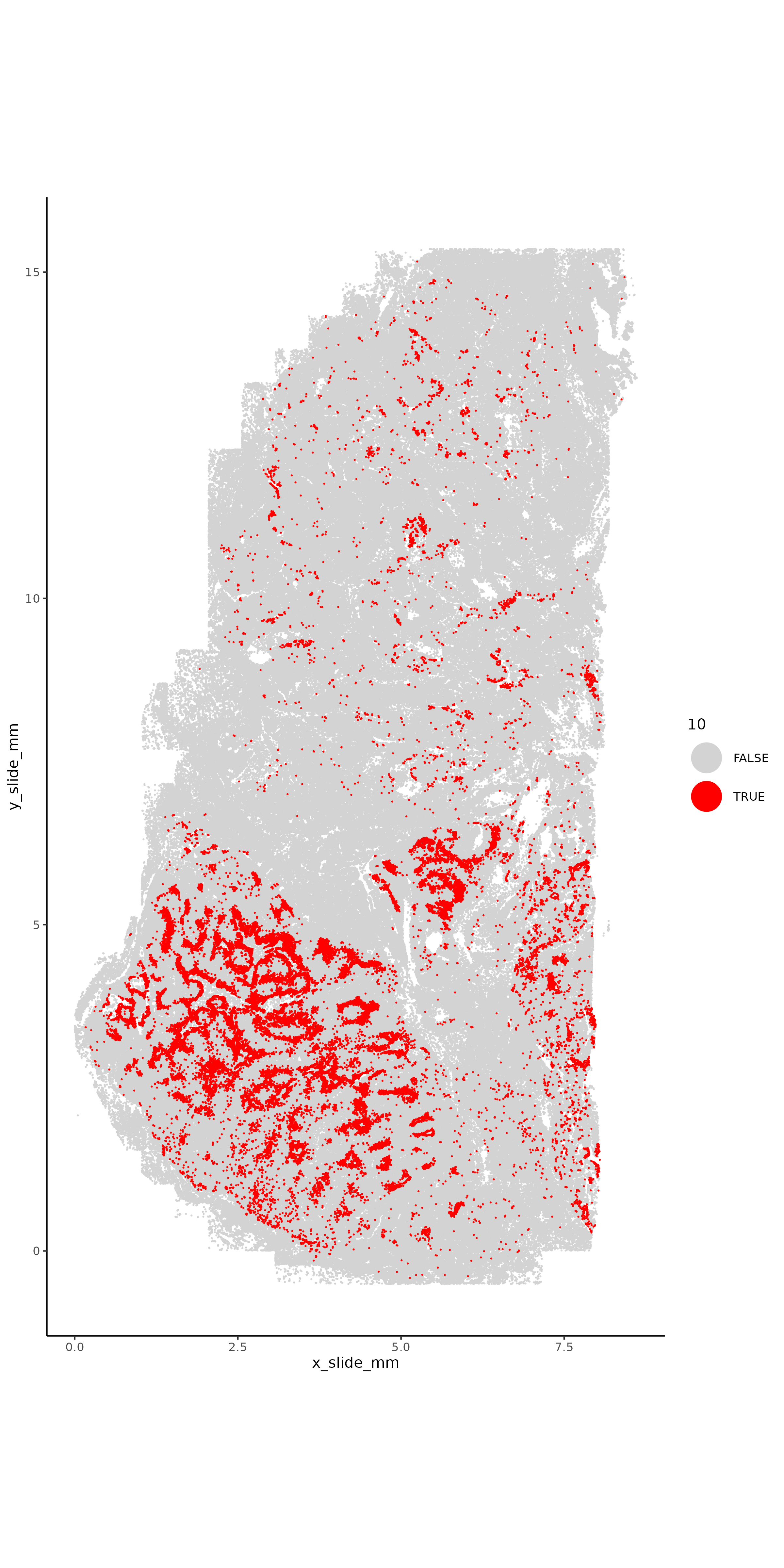
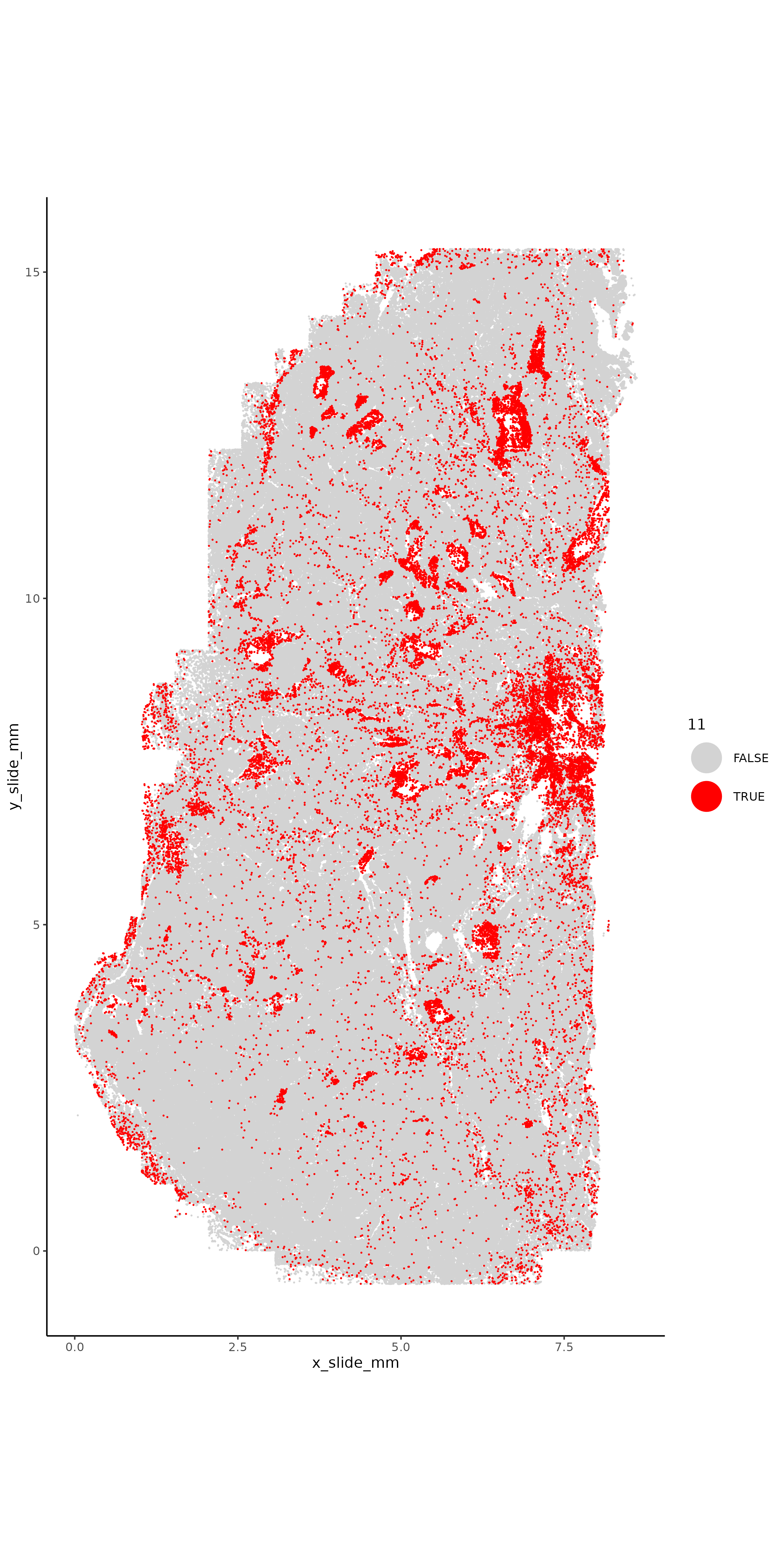
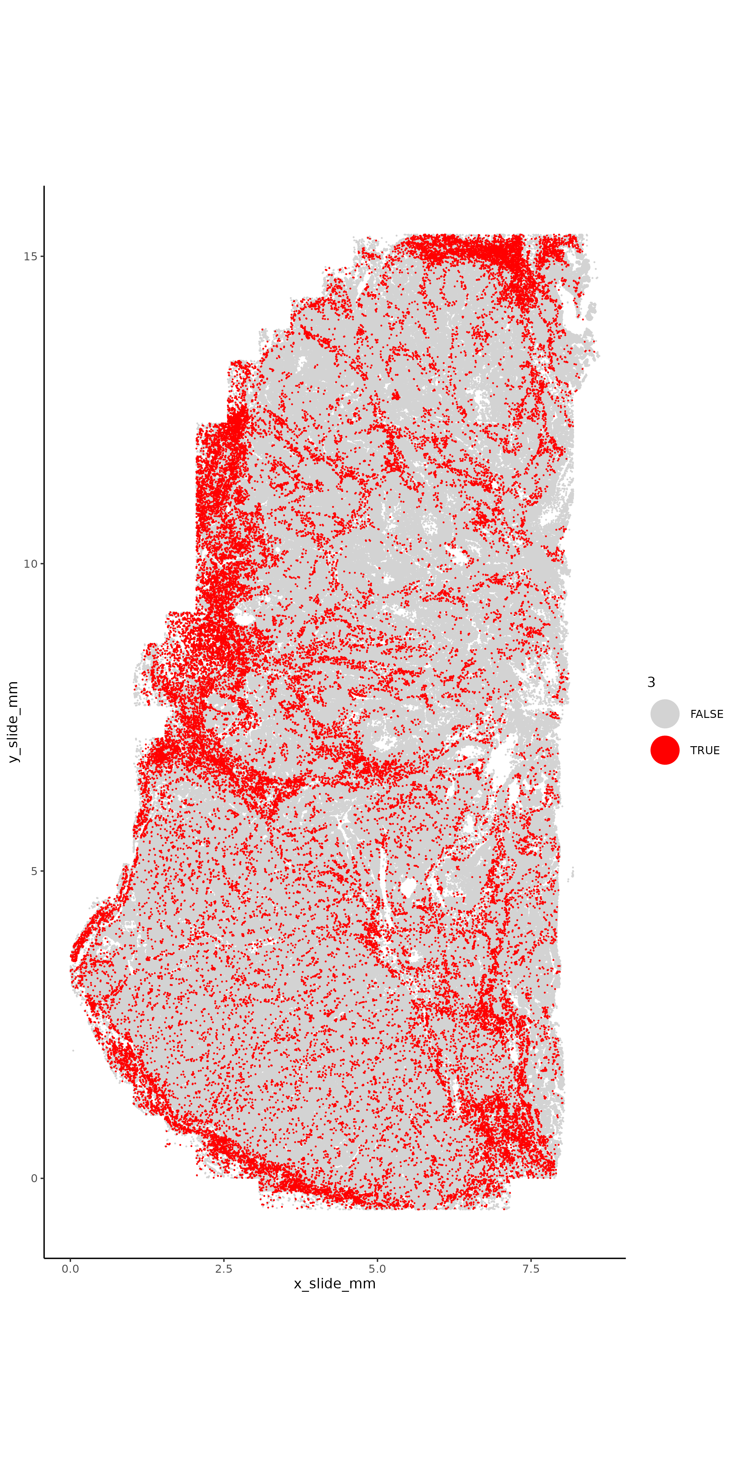
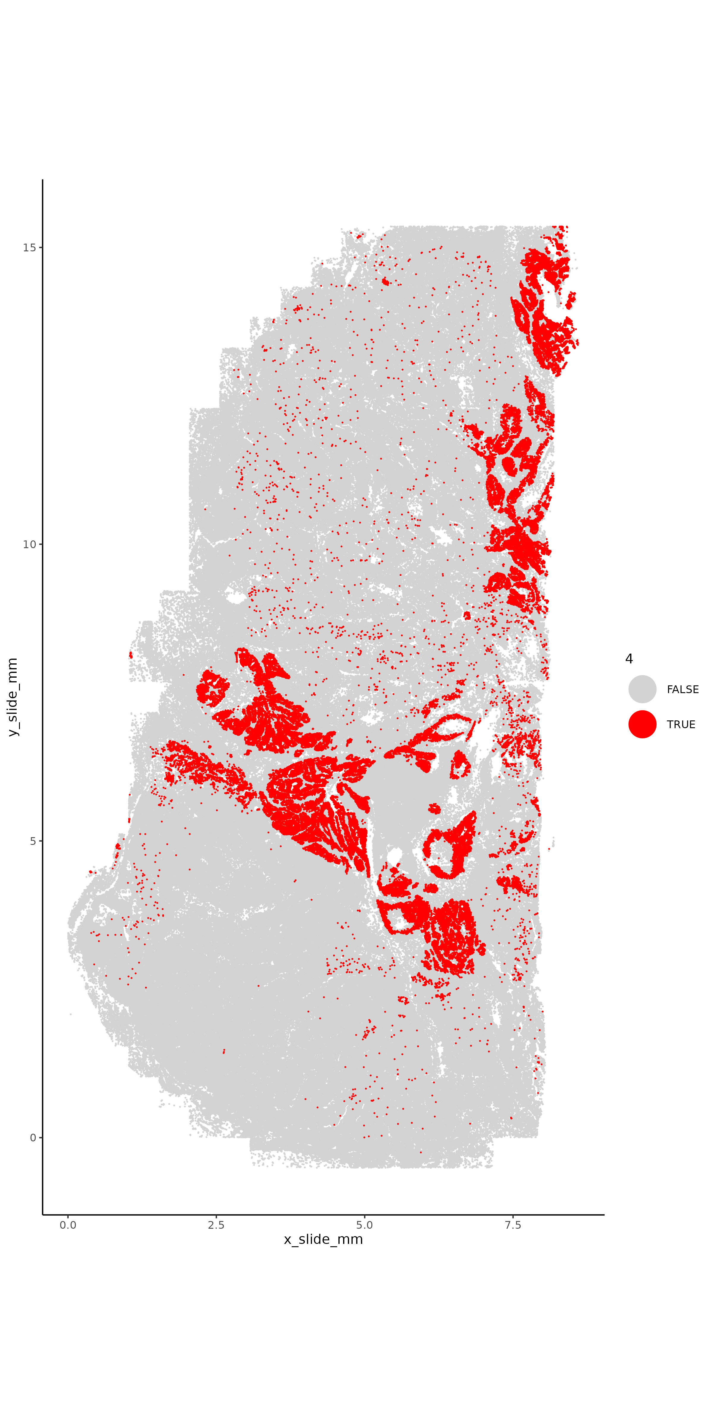
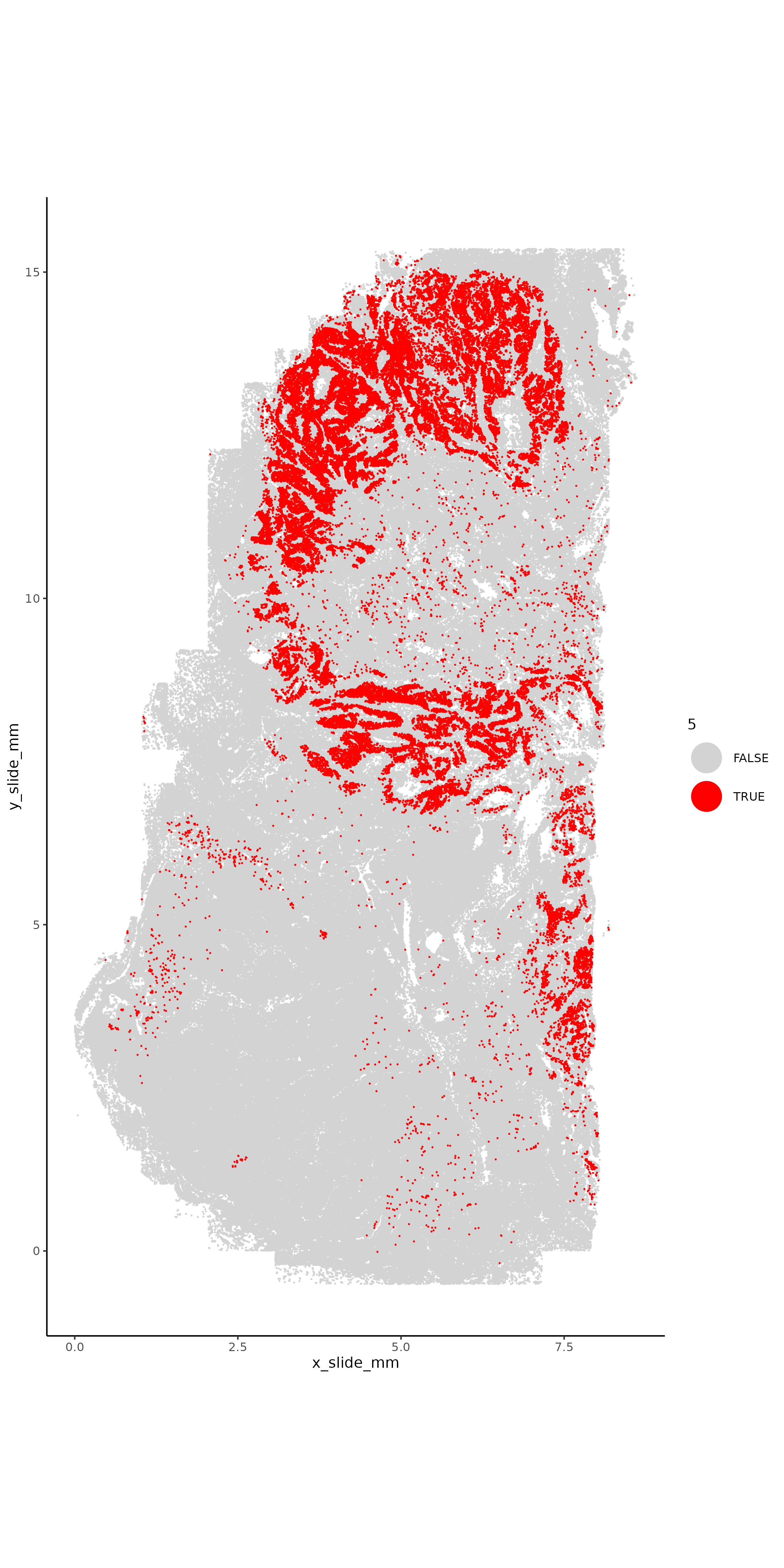
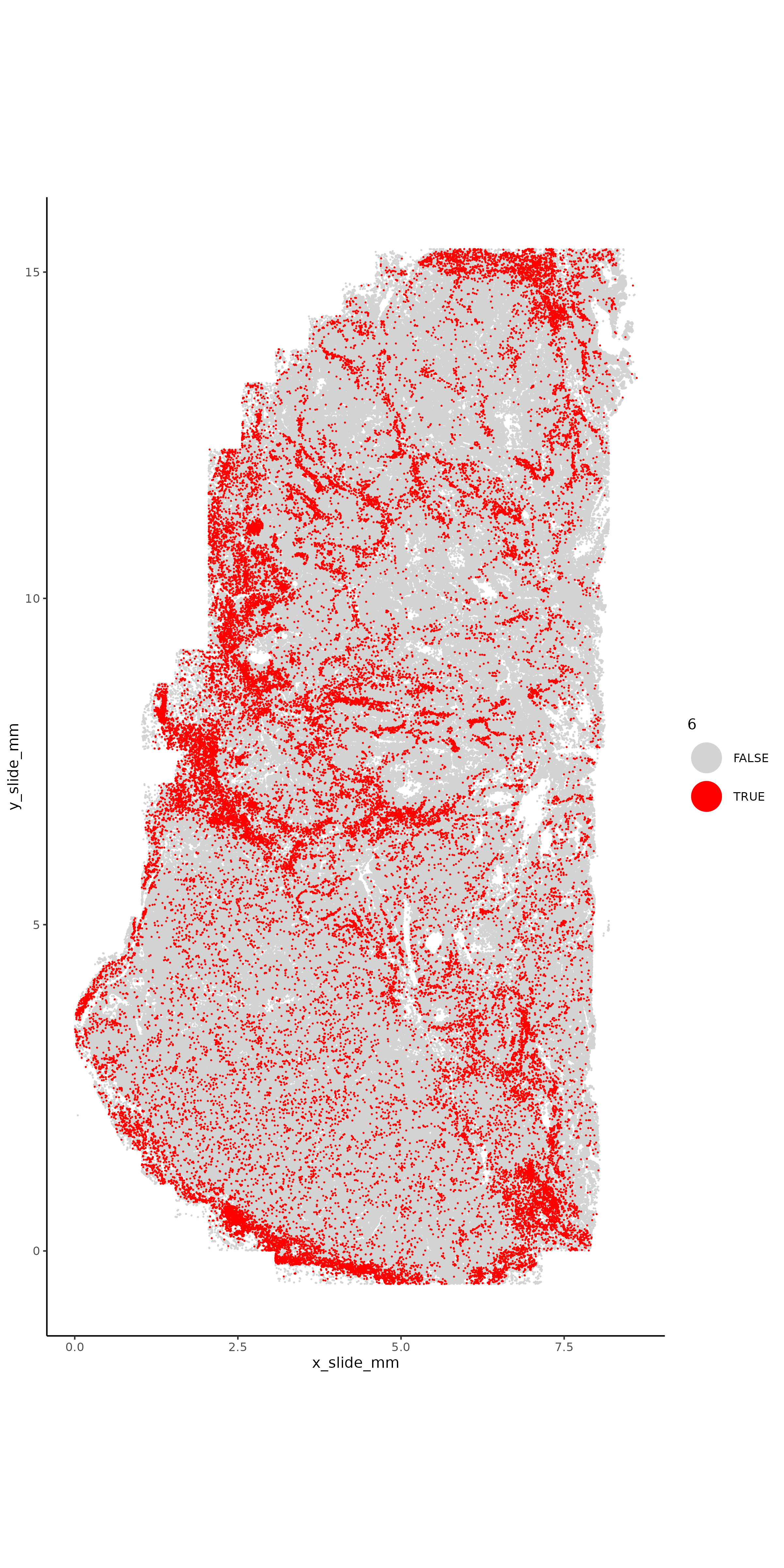
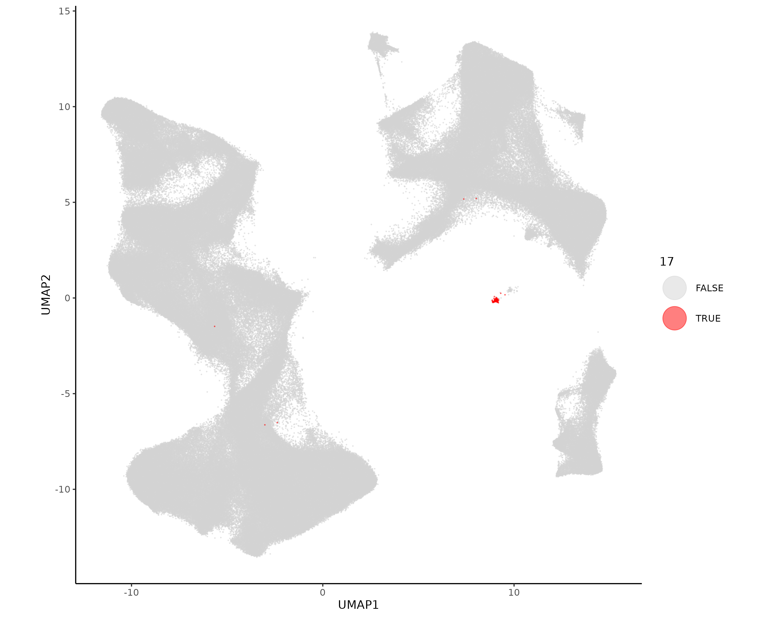
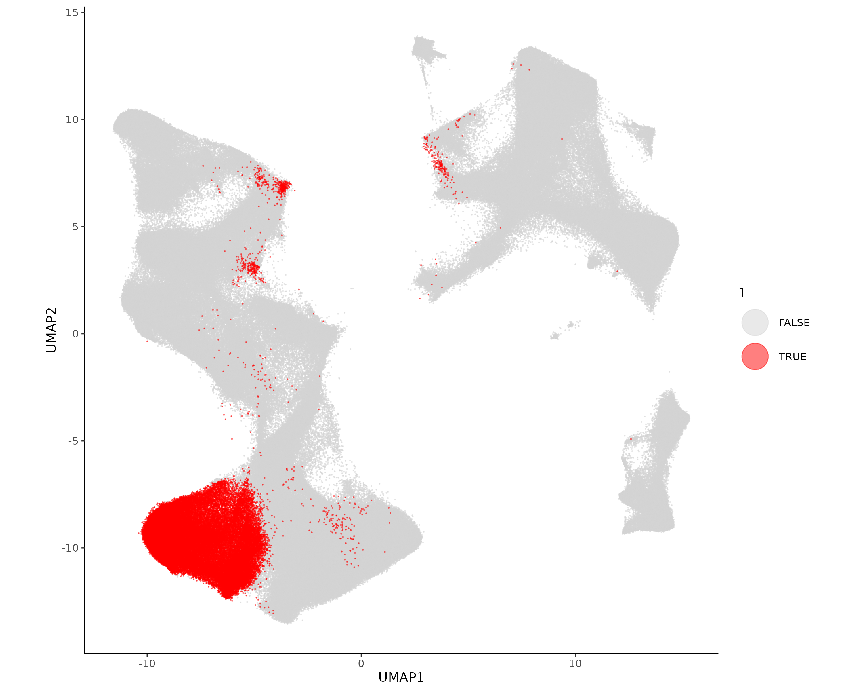
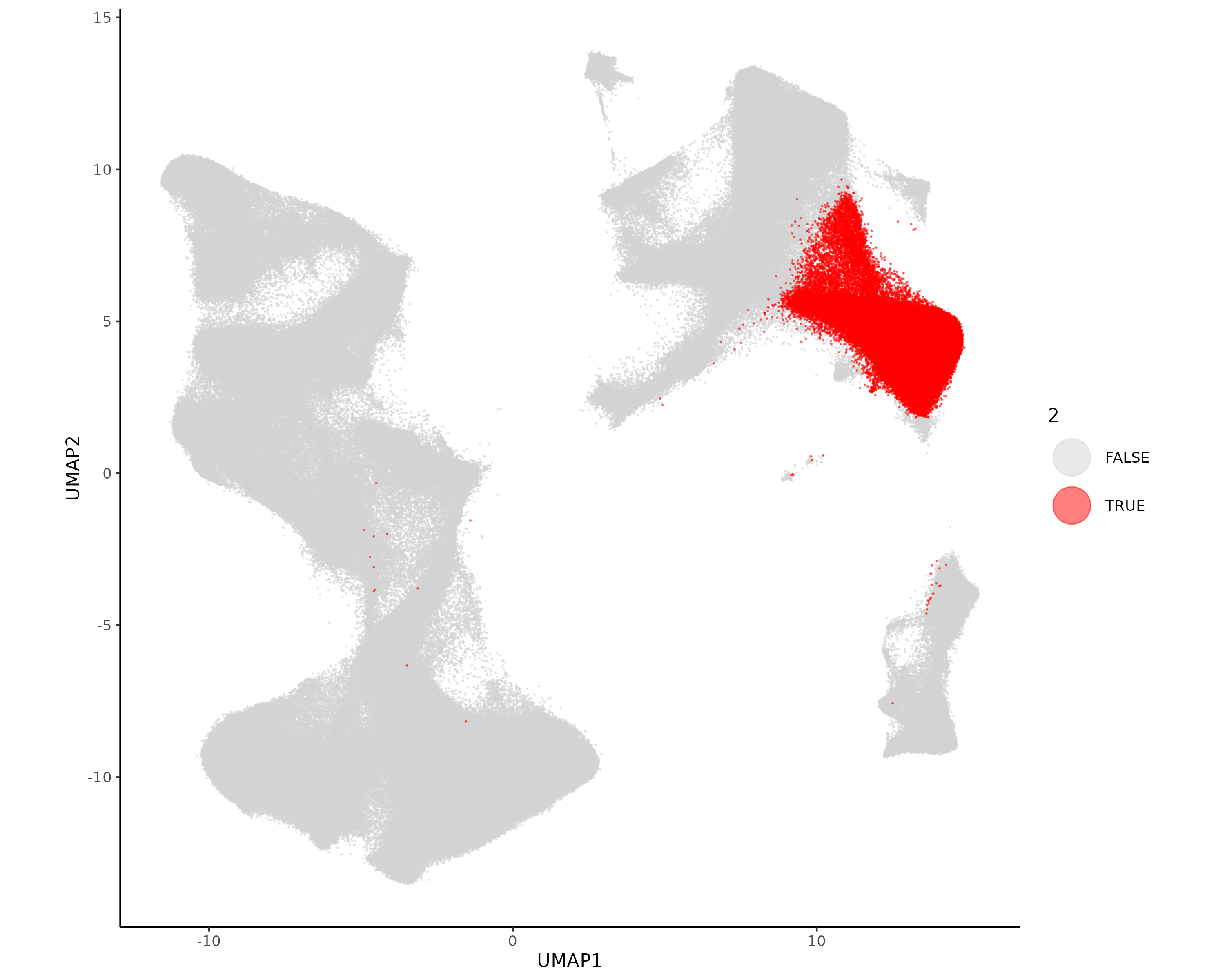
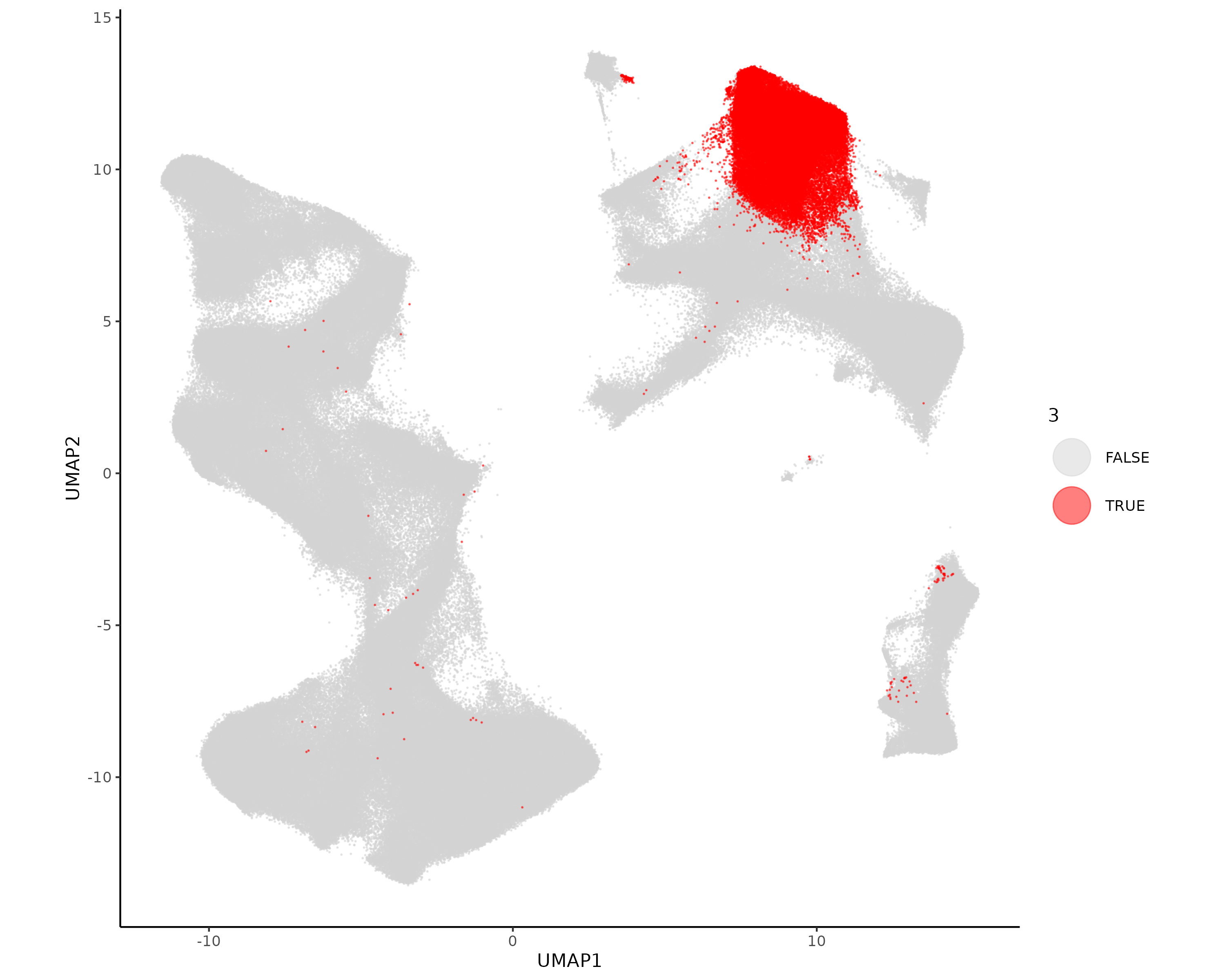
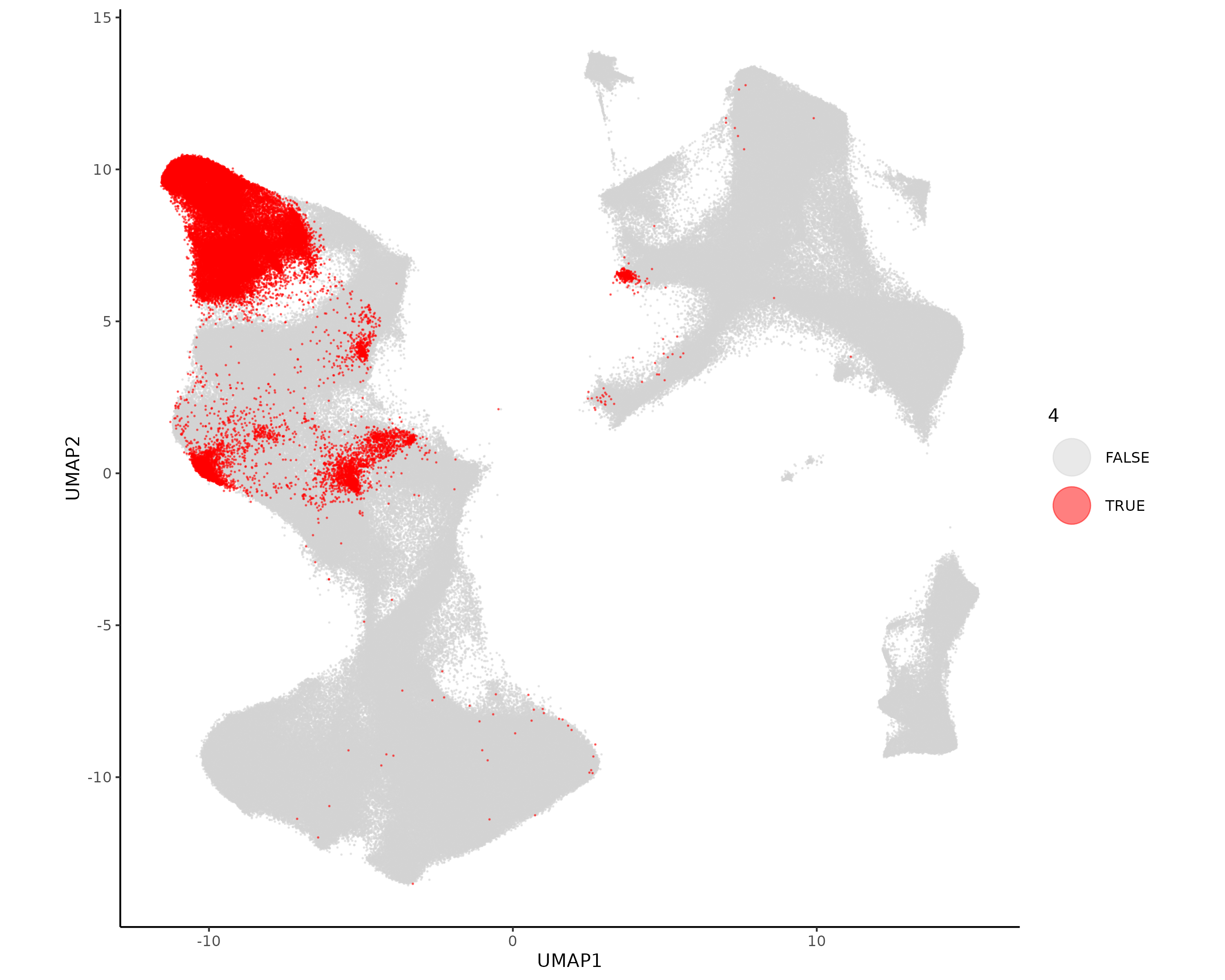
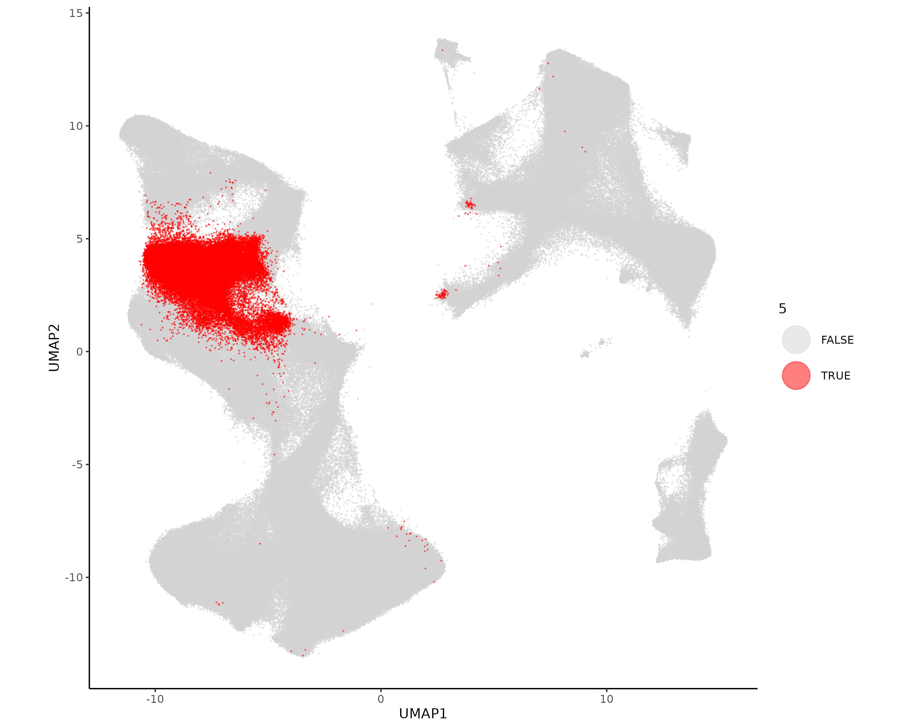
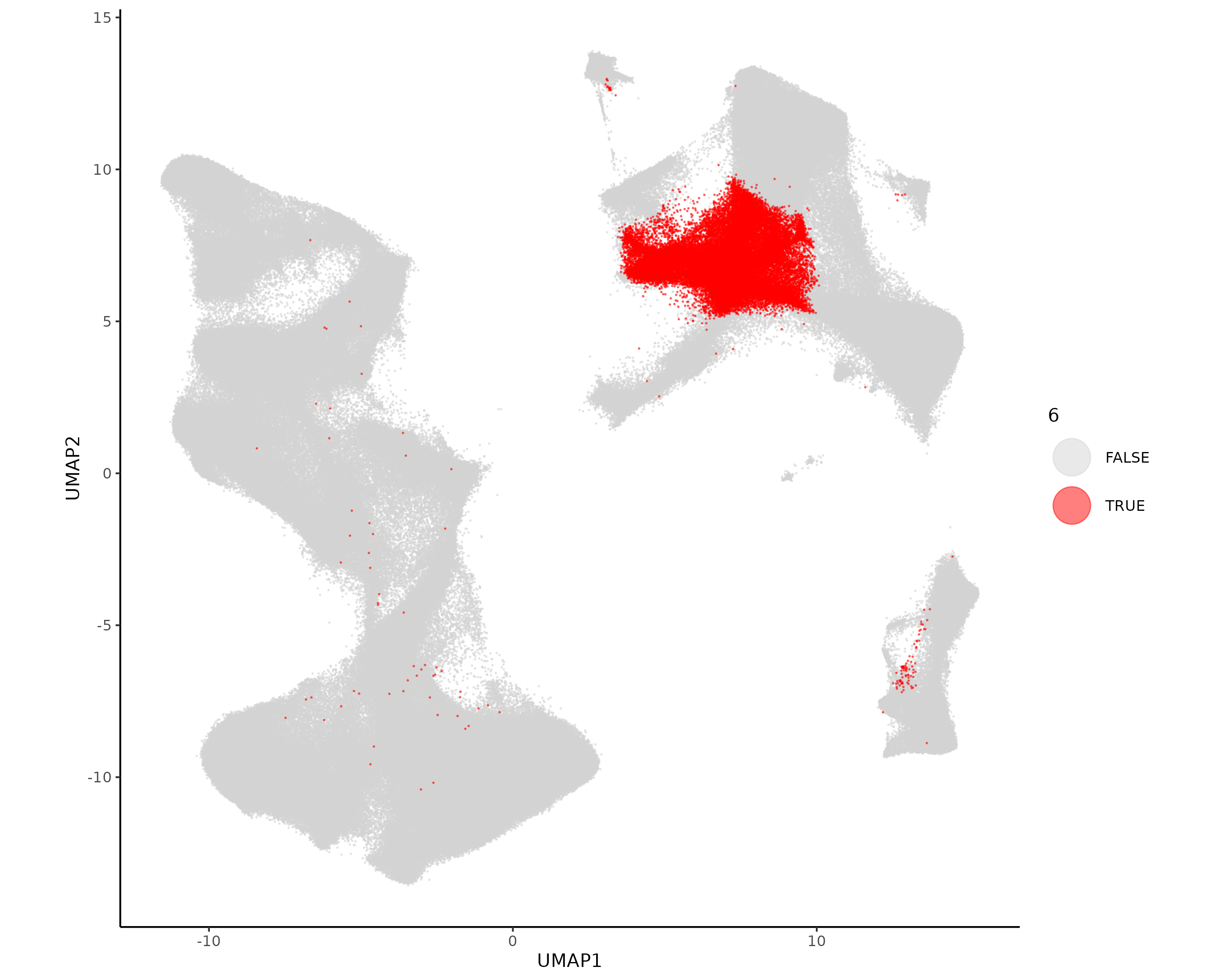
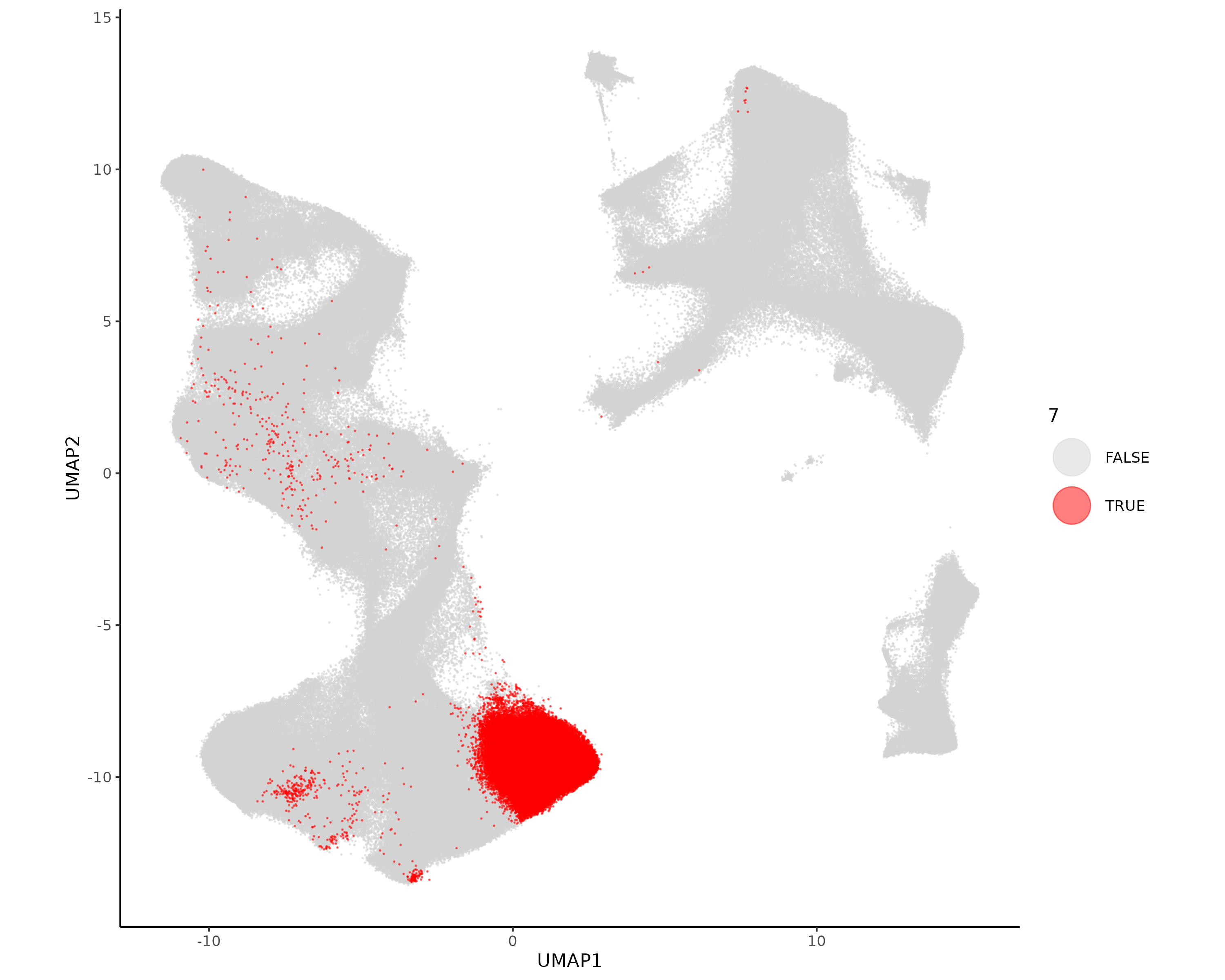
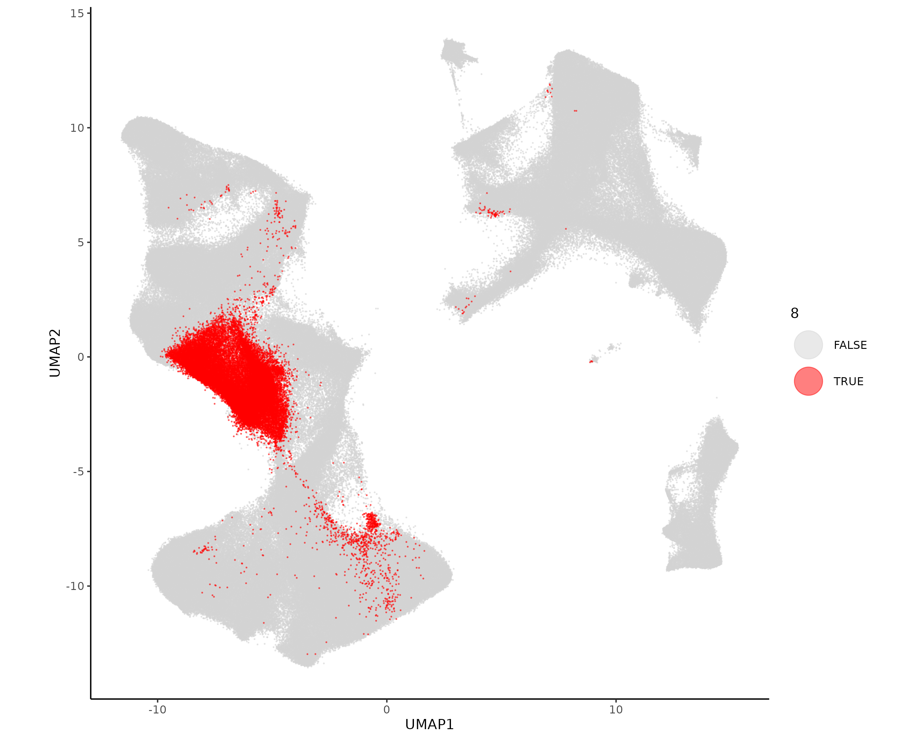
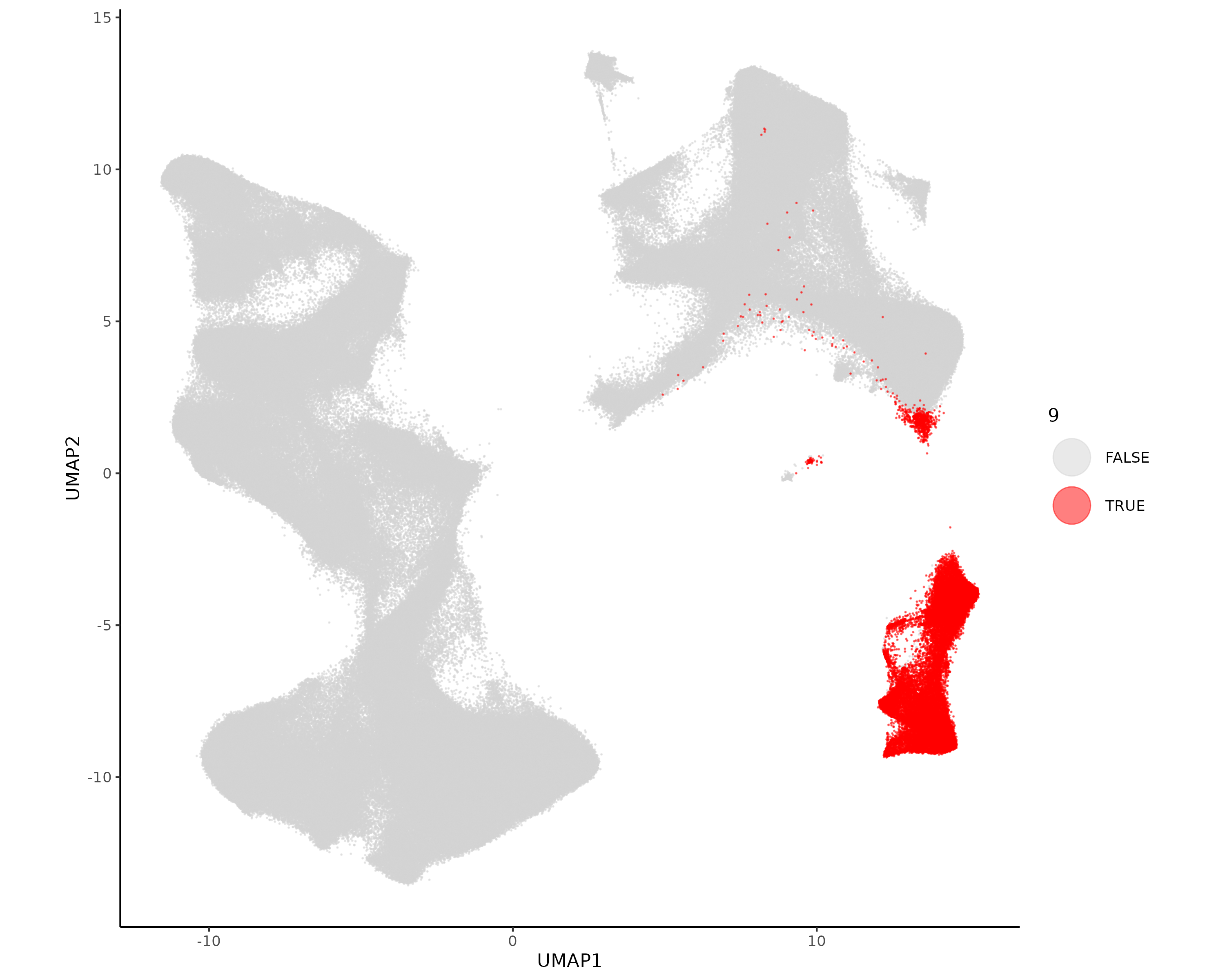
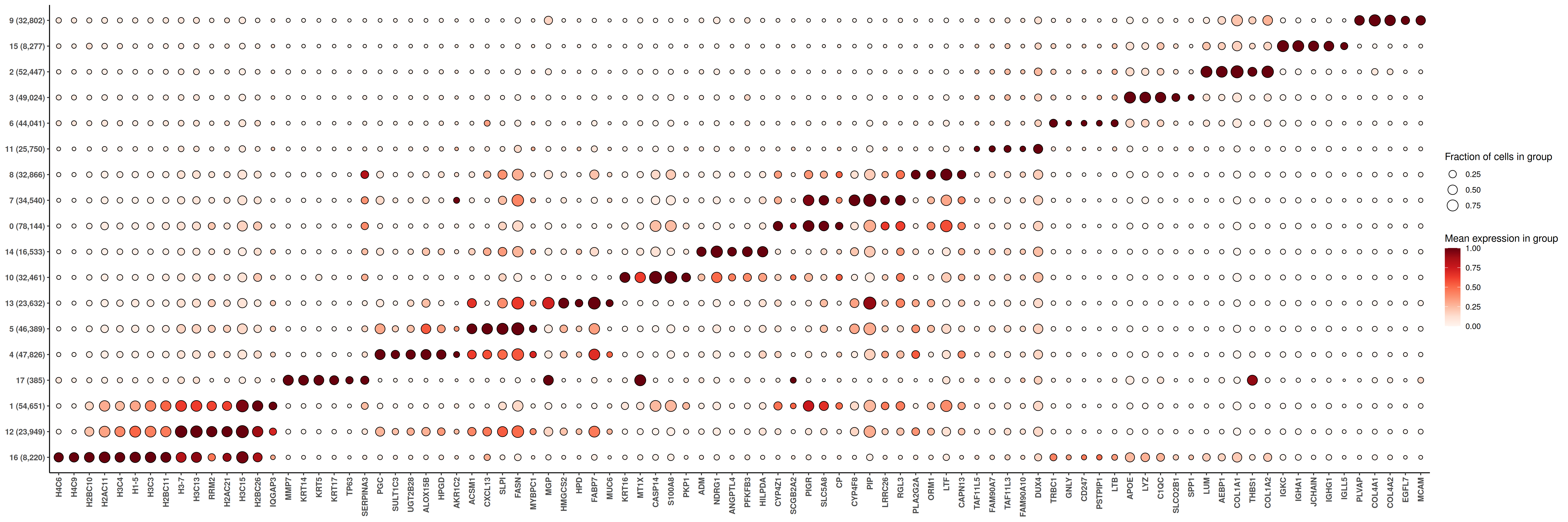
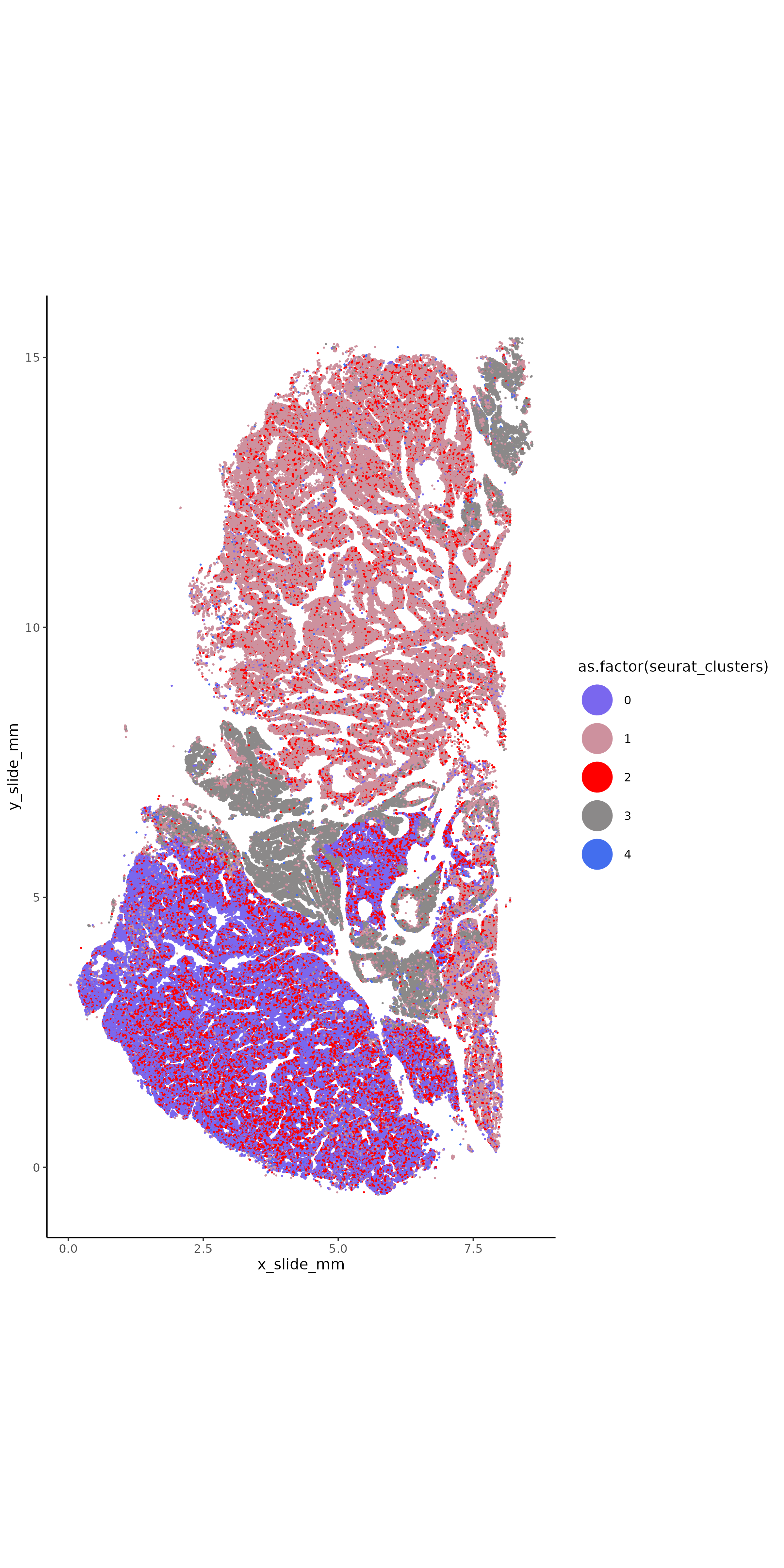
if (!("seu.obj"%in%ls())){ seu.obj <-readRDS(results_list$seurat_file_postUMAP)}# With Seuratseu.obj <- Seurat::FindClusters(seu.obj, graph.name ="umapgrph", resolution =0.7)# Plot it in XY space with random colorsset.seed(2024)my_pal <-sample(colors(distinct =TRUE), length(unique(seu.obj@meta.data$seurat_clusters)))names(my_pal) <-as.character(unique(seu.obj@meta.data$seurat_clusters))ggplot(seu.obj@meta.data,aes(x = x_slide_mm, y = y_slide_mm, color =as.factor(seurat_clusters))) +geom_point(size =0.1) +scale_color_manual(values = my_pal) +theme_classic() +coord_fixed() +guides(colour =guide_legend(override.aes =list(size=10)))ggsave(filename =paste0(dimRed_dir, "/Plots/XY_leiden.png"),width =8, height =16, units ="in")# Plot each cell type separatelyfor (ct inunique(seu.obj@meta.data$seurat_clusters)){ggplot(seu.obj@meta.data[order(seu.obj@meta.data$seurat_clusters == ct),],aes(x = x_slide_mm, y = y_slide_mm, color = seurat_clusters==ct)) +geom_point(size =0.05) +scale_color_manual(values =c("lightgrey", "red"), name = ct) +theme_classic() +coord_fixed() +guides(colour =guide_legend(override.aes =list(size=10)))ggsave(filename =paste0(dimRed_dir, "/Plots/XY_leiden_", ct, ".png"),width =8, height =16, units ="in")}# Plot it in UMAP spaceDimPlot(seu.obj, group.by ="seurat_clusters", reduction ="umap", label = T) +scale_color_manual(values = my_pal)ggsave(filename =paste0(dimRed_dir, "/Plots/umap_leiden.png"))# Plot each cell type separately in UMAP spaceplot.df <- seu.obj@meta.dataplot.df$UMAP1 <- seu.obj@reductions$umap@cell.embeddings[,1]plot.df$UMAP2 <- seu.obj@reductions$umap@cell.embeddings[,2]for (ct inunique(plot.df$seurat_clusters)){ggplot(plot.df[order(plot.df$seurat_clusters == ct),],aes(x = UMAP1, y = UMAP2, color = seurat_clusters==ct)) +geom_point(size =0.05, alpha =0.5) +scale_color_manual(values =c("lightgrey", "red"), name = ct) +theme_classic() +coord_fixed() +guides(colour =guide_legend(override.aes =list(size=10)))ggsave(filename =paste0(dimRed_dir, "/Plots/UMAP_leiden_", ct, ".png"),width =10, height =8, units ="in")}# Generate a marker heatmap with HieraType functions## prepare data for marker gene heatmap:fc_subclus_ctl_gran <-clusterwise_foldchange_metrics(seu.obj[["RNA"]]@counts ,metadata = seu.obj@meta.data ,cluster_column ="seurat_clusters")# subtract background from the mean per-cluster expression profiles:neg_counts <- seu.obj@assays$negprobes$countsfor (name inunique(seu.obj@meta.data$seurat_clusters)) { isthiscelltype <- seu.obj@meta.data$seurat_clusters == name meannegthiscelltype <- Matrix::mean(neg_counts[, isthiscelltype]) fc_subclus_ctl_gran$cluster_expr[fc_subclus_ctl_gran$cluster == name] <-pmax(fc_subclus_ctl_gran$cluster_expr[fc_subclus_ctl_gran$cluster == name] - meannegthiscelltype, 0)}# create the heatmap:hm_semiSup <-add_ncells(marker_heatmap(fc_subclus_ctl_gran))png(filename =paste0(dimRed_dir, "/Plots/heatmap_leiden_negRemoved.png"),width =24, height =8, units ="in", res =300)print(hm_semiSup)dev.off()# Save seurat objectresults_list$leiden_color_pal <- my_palresults_list$seurat_file_postLeiden <-paste0(objects_dir, "/seurat_object_postLeiden.rds")saveRDS(results_list, results_list_file)saveRDS(seu.obj, results_list$seurat_file_postLeiden)
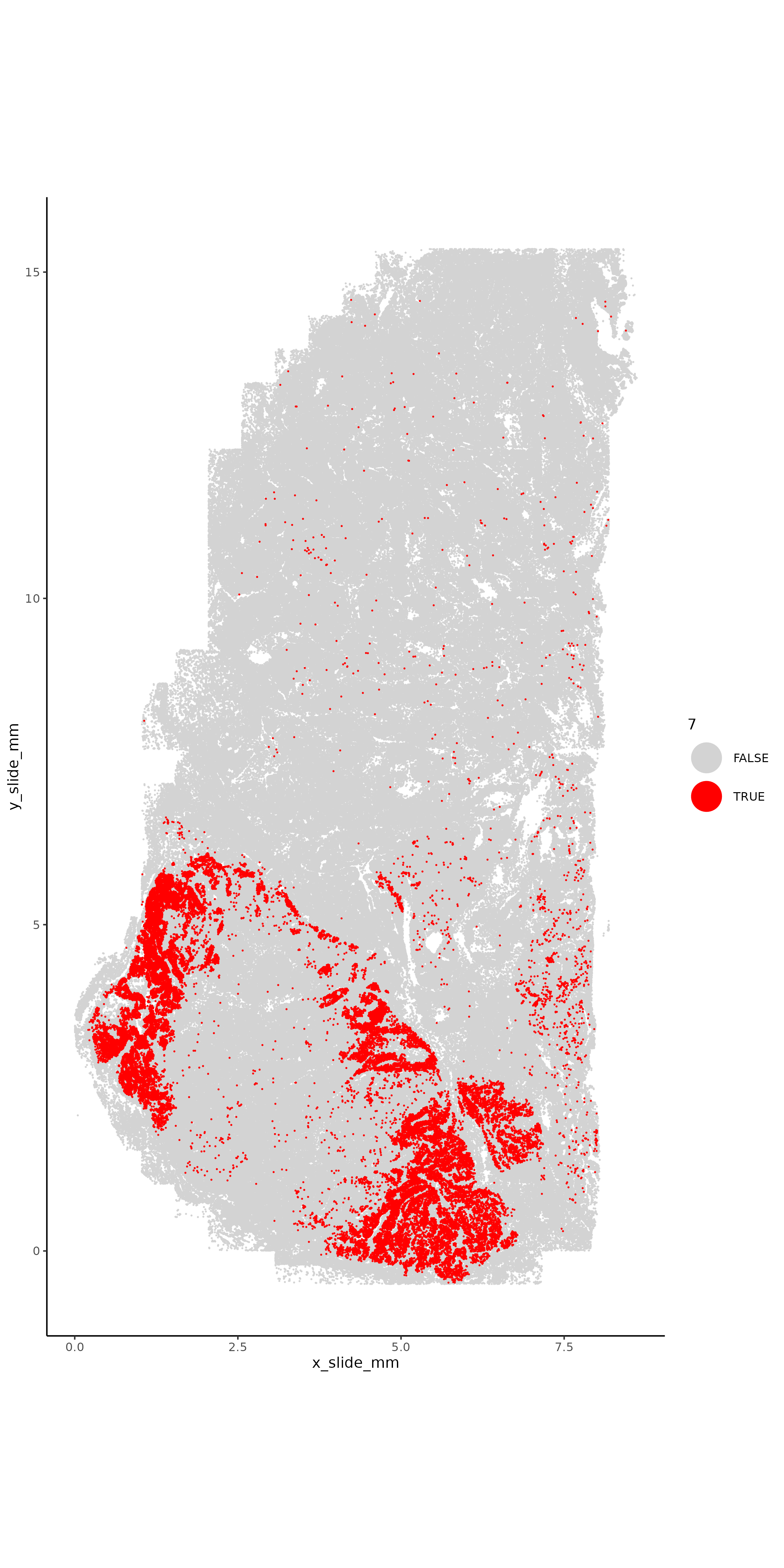
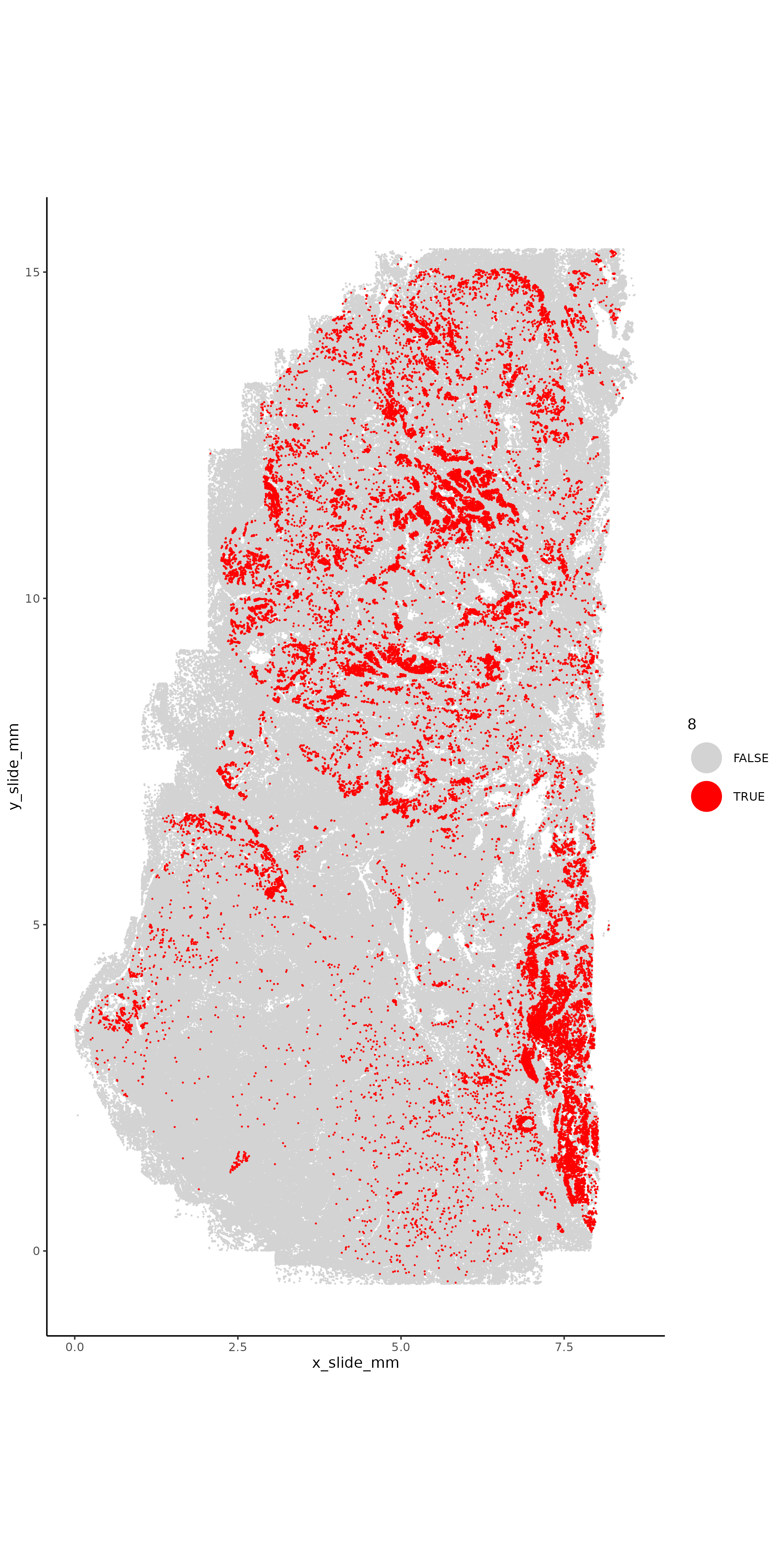
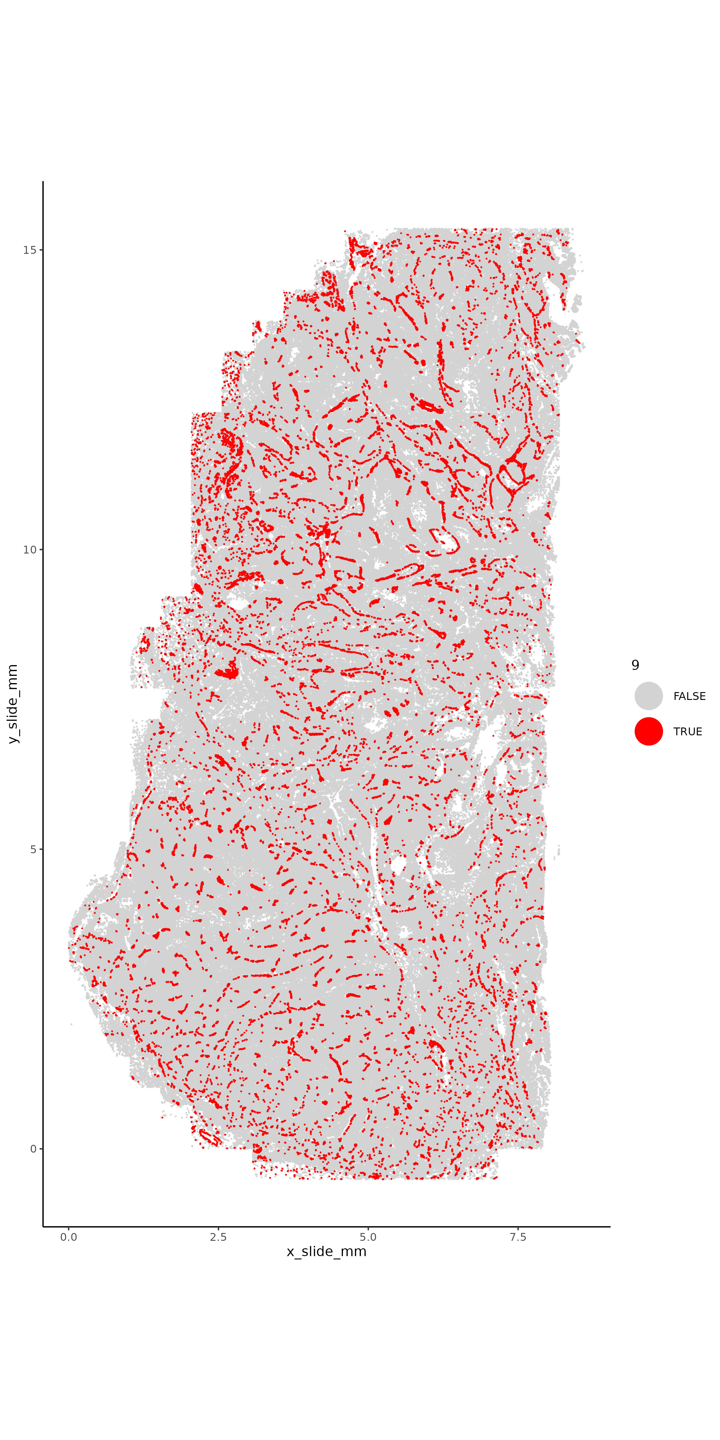
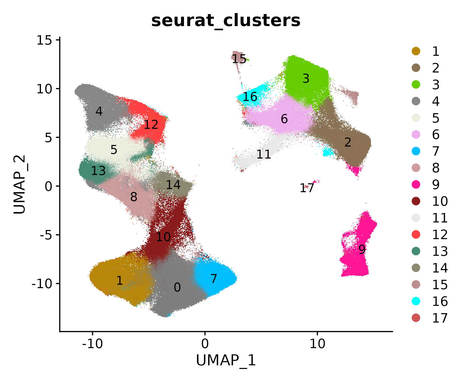
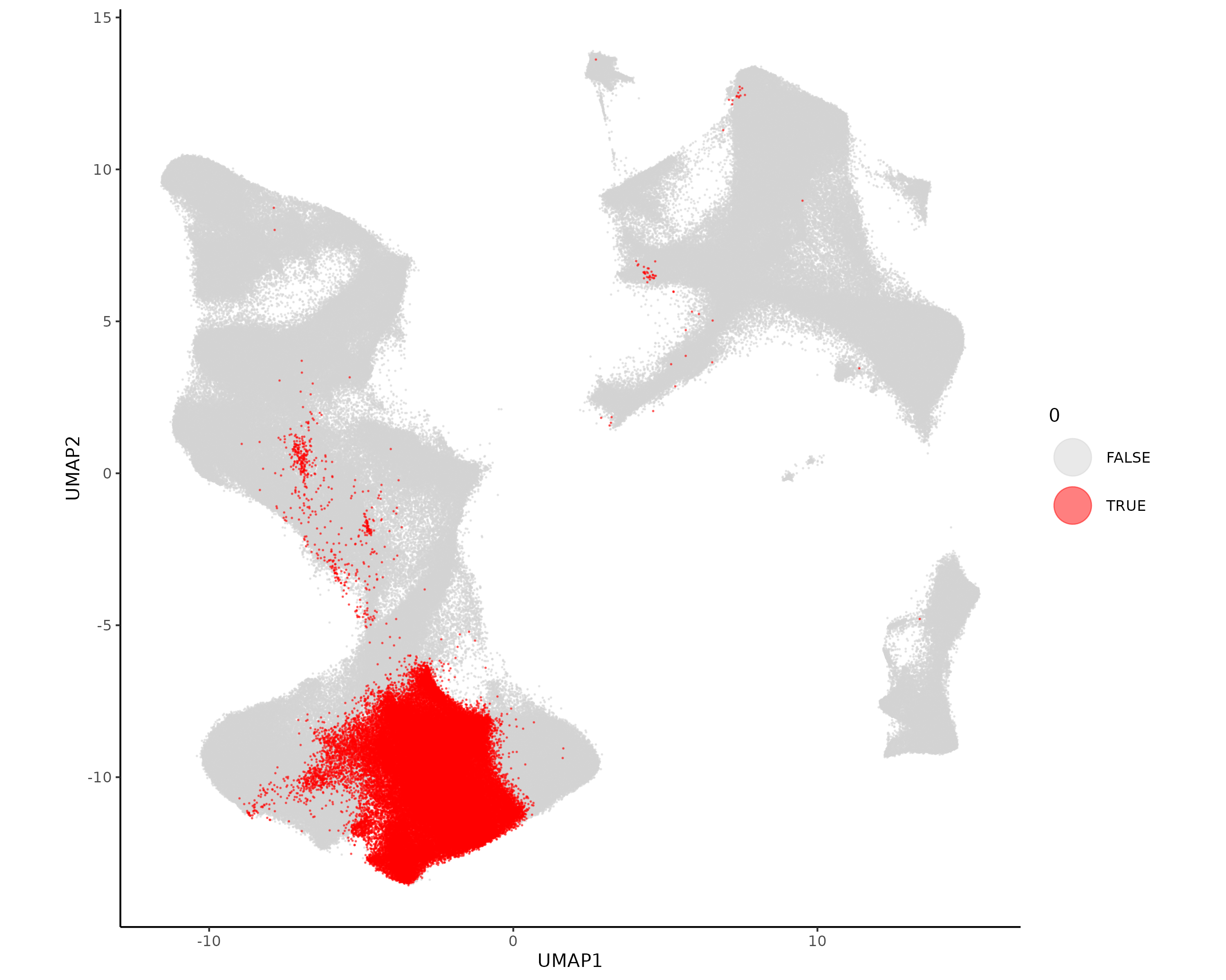
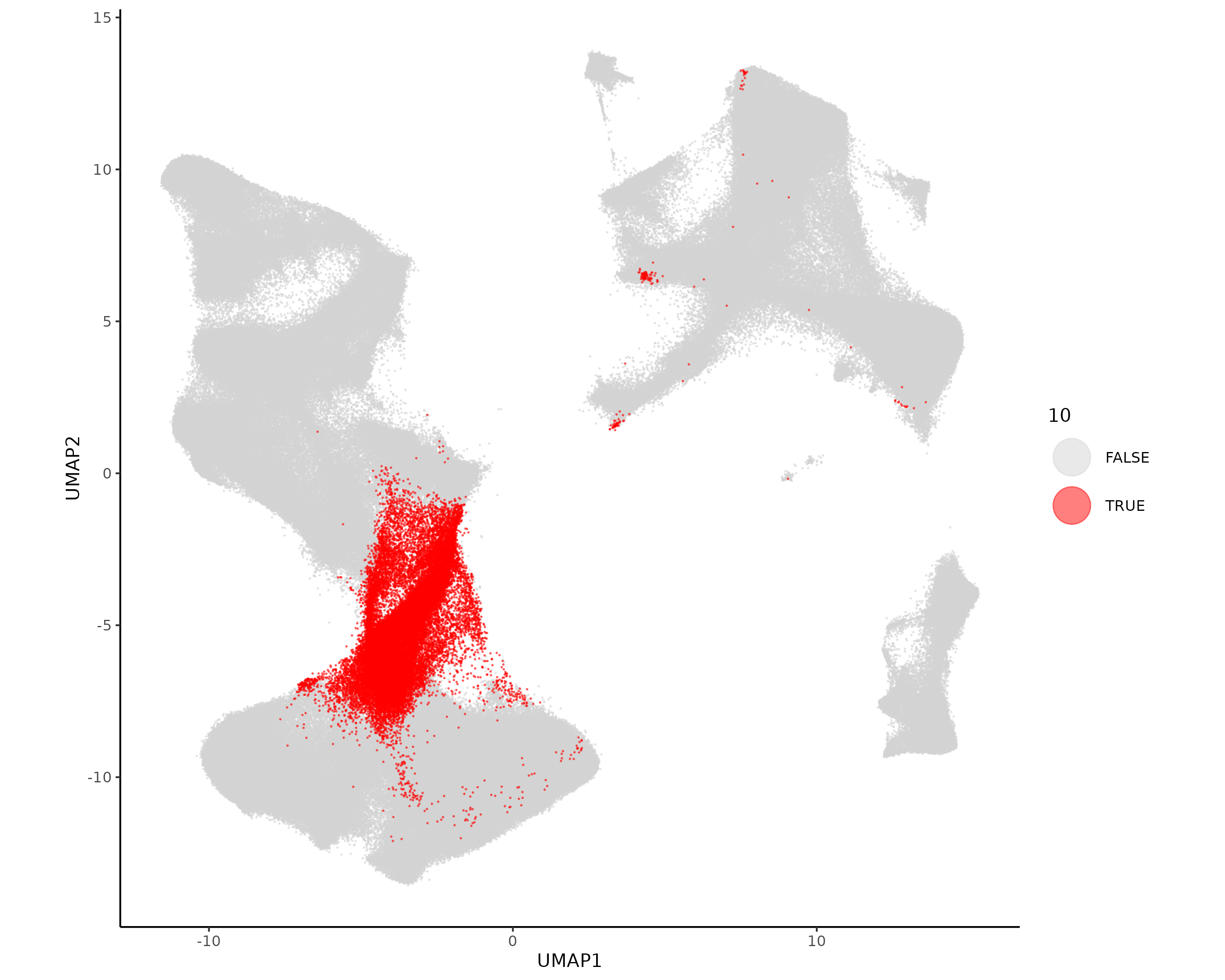
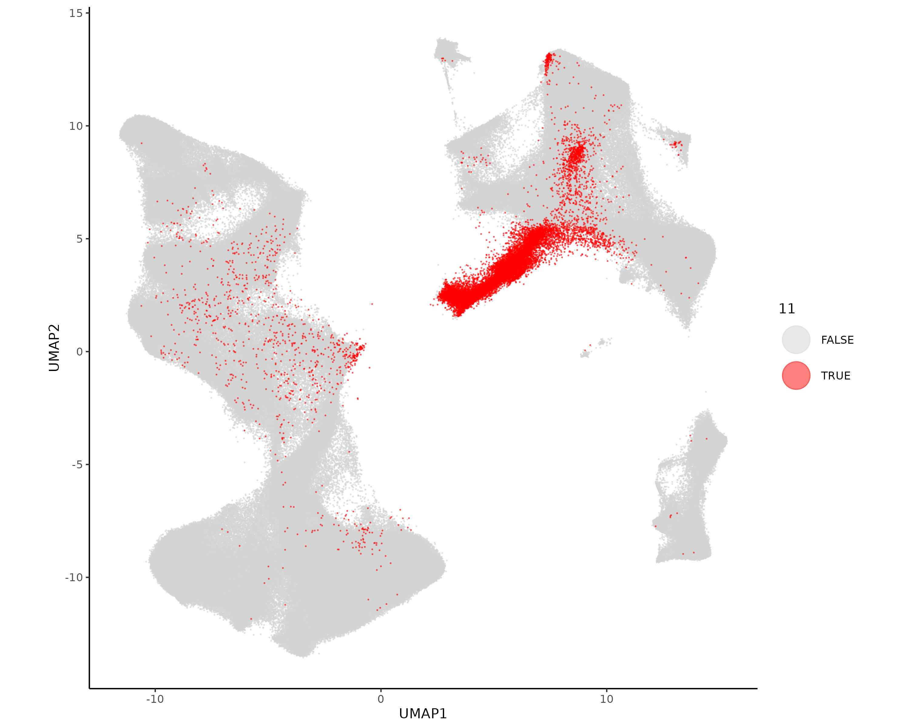
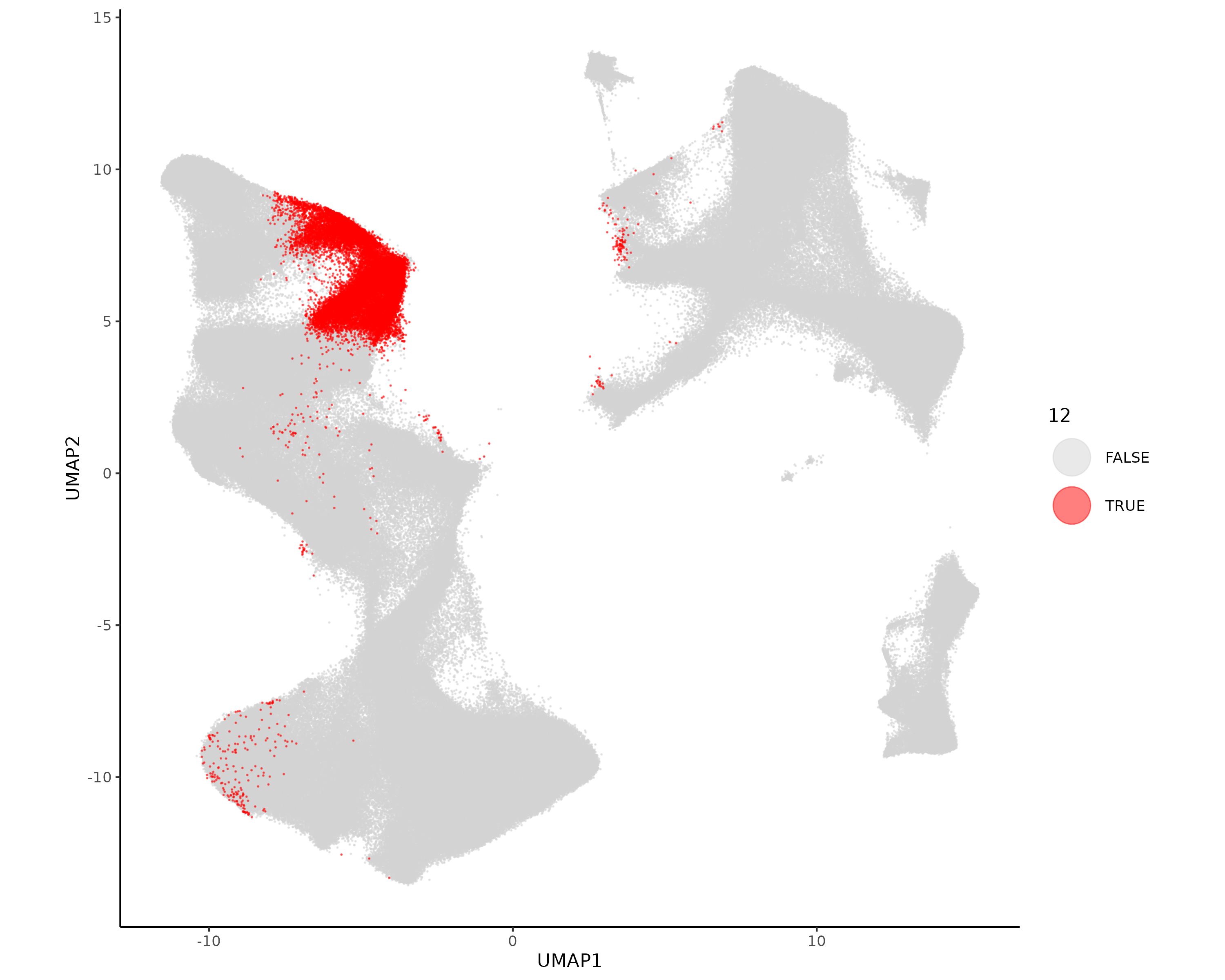
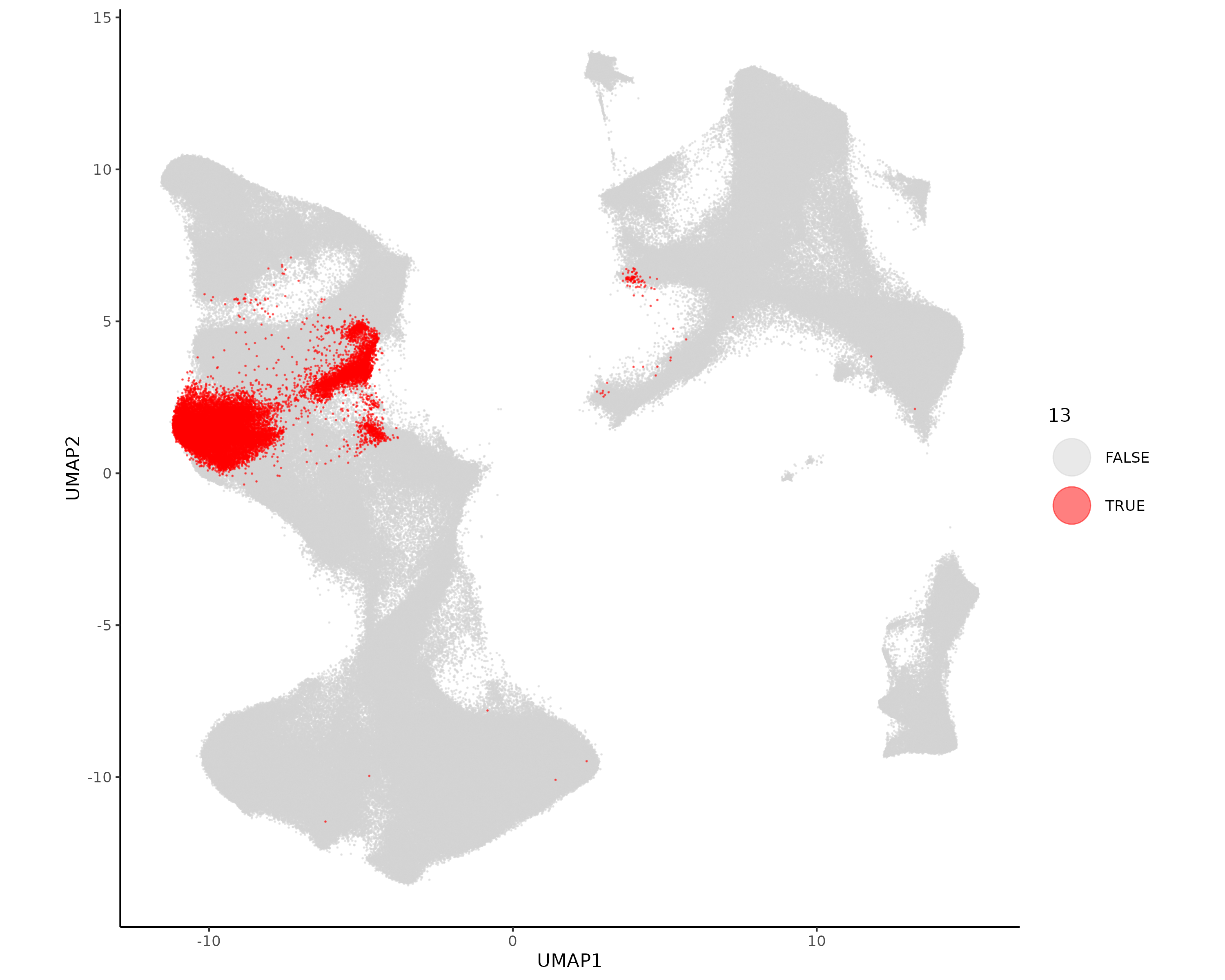
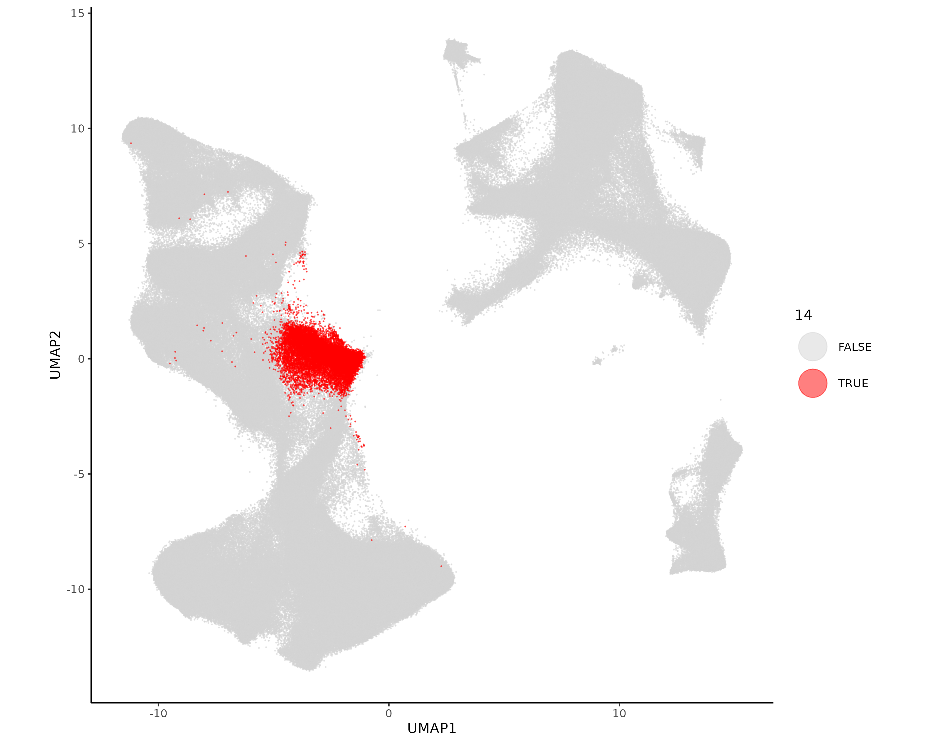
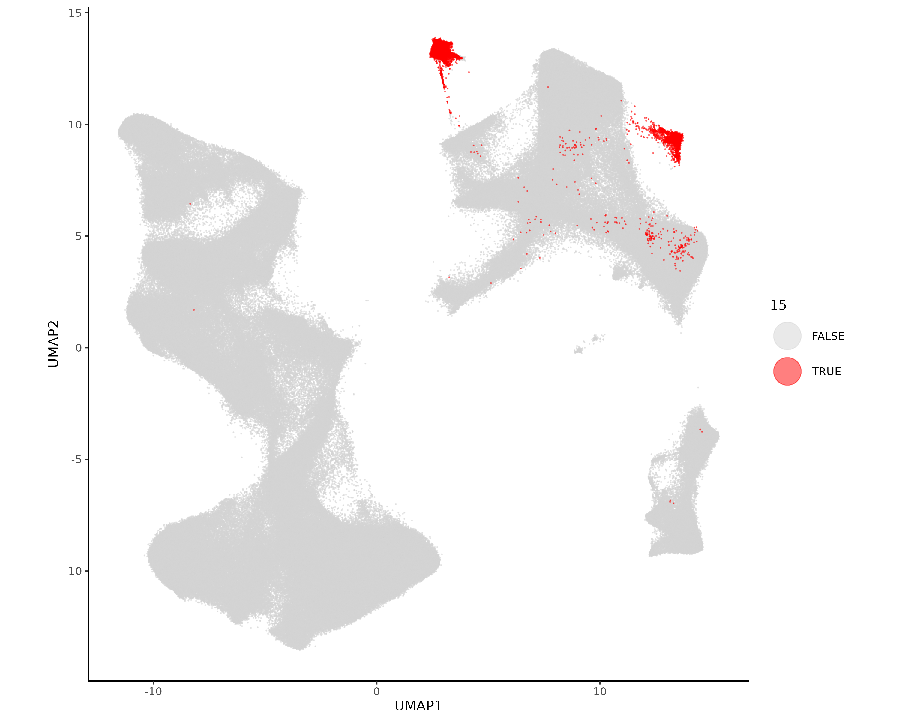
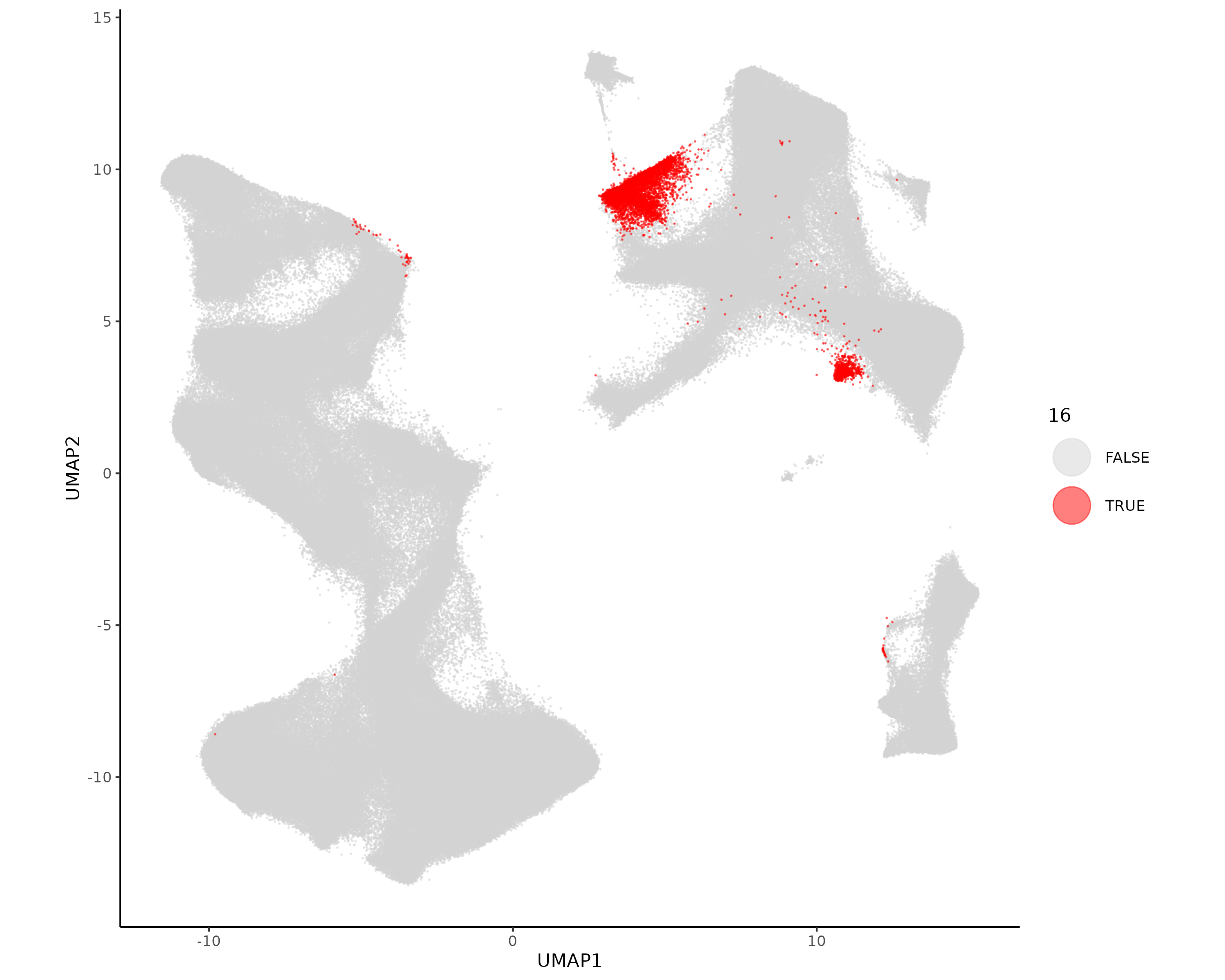
These unsupervised clusters do a pretty good job of splitting apart major cell types. We follow this up by naming and refining this initial clustering result based on spatial distribution, top marker genes, and position in UMAP space. In particular, we’ll recluster the tumor cells on their own to reduce the number of clusters and subcluster the fibroblast and vascular clusters. Additionally, we’ll use HieraType to perform targeted marker-based annotation of the immune cells. We start with our evaluation and planned actions for each cluster:
Cell type
Evaluation
Refinement
0
Tumor, lower lobe
Tumor recluster
1
Tumor, lower lobe
Tumor recluster
2
Fibroblasts, markers LUM, THBS1, AEBP1
Fibroblast subcluster
3
Immune, myeloid
Immune HieraType
4
Tumor, between lobes
Tumor recluster
5
Tumor, exterior of upper lobe
Tumor recluster
6
Immune
Immune HieraType
7
Tumor, exterior of lower lobe
Tumor recluster
8
Tumor, spotty
Tumor recluster
9
Vasculature
Vasculature subcluster
10
Tumor, lower lobe
Tumor recluster
11
Low count cells near tissue gaps. Necrotic cells.
Rename necrotic cells
12
Tumor, upper lobe
Tumor recluster
13
Tumor, interior of upper lobe
Tumor recluster
14
Tumor, adjacent to necrotic zones
Tumor recluster
15
Plasma cells two clusters in UMAP space
Immune HieraType
16
Immune, proliferative
Immune HieraType
17
Small number of border cells and well defined small clusters, potentially healthy epithelia
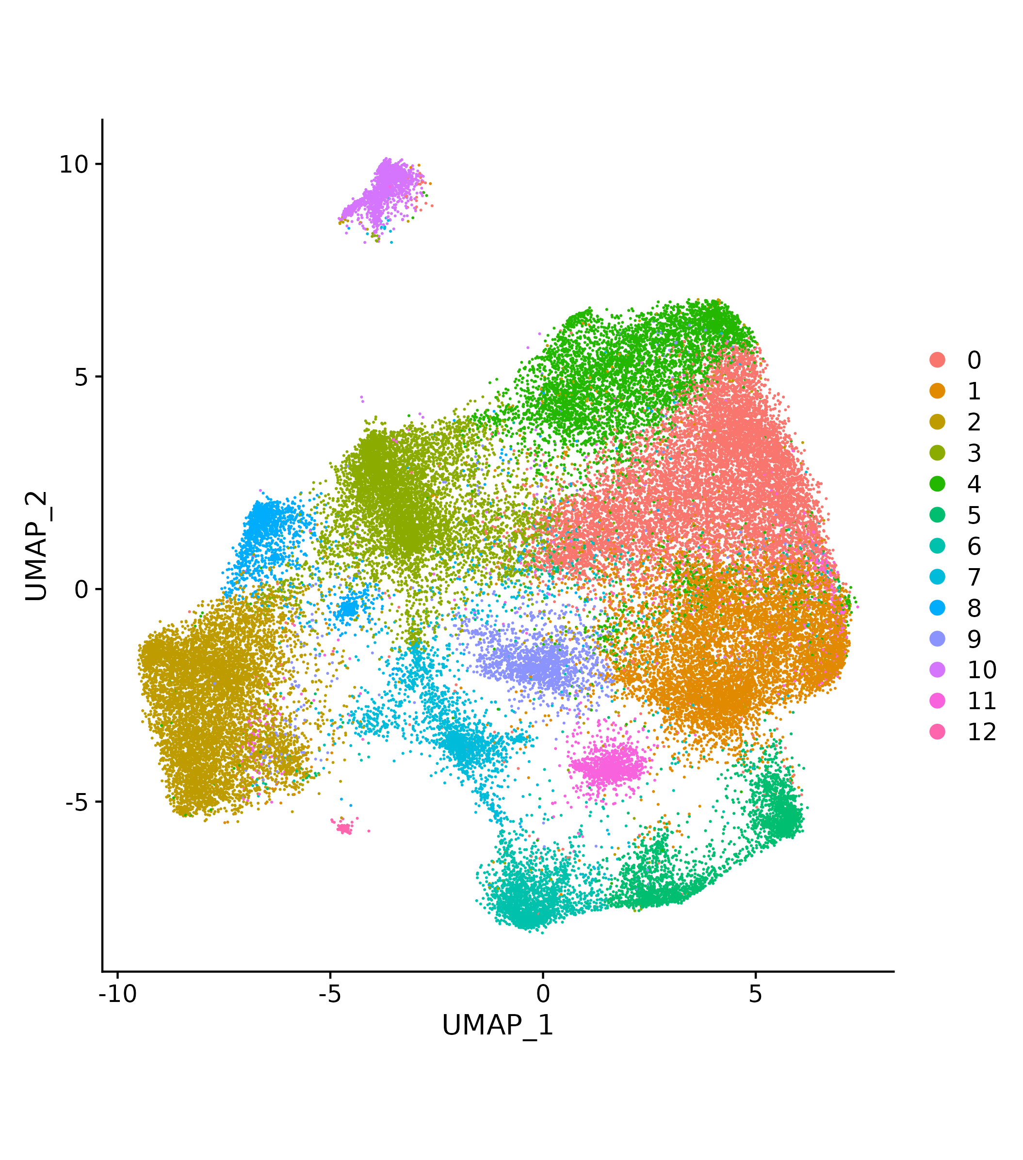
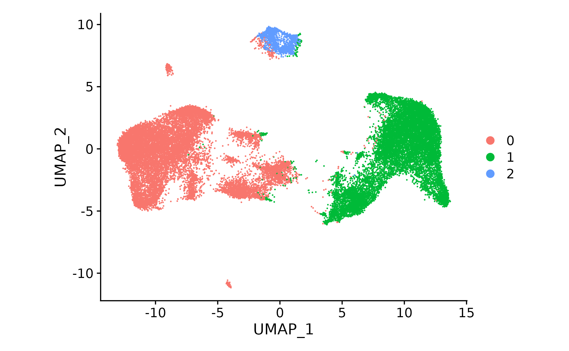
We start with fibroblasts since this cluster is near immune clusters and may be partially overlapping. The initial unsupervised clustering had only one fibroblast cluster, but from previous experience with this sample we expect that we should be able to identify a few subtypes. Additionally, it appears that the cluster that is mostly fibroblast may also contain some immune cells. Here we take the fibroblast cells, repeat initial preprocessing so that highly variable genes are chosen based on these cells, and use unsupervised clustering to separate these cells into multiple clusters, some of which we’ll add to the immune cells for HieraType clustering.
Show the code
if (!("seu.obj"%in%ls())){ seu.obj <-readRDS(results_list$seurat_file_postLeiden)}# Subset the seurat object to only include fibroblast clusterfibro_leiden <-c(2)fibro_idx <-which(seu.obj@meta.data$seurat_clusters %in% fibro_leiden)seu.fibro <- seu.obj[,fibro_idx]# Repeat preprocessing, dimension reduction, and leiden clusteringseu.fibro <-NormalizeData(seu.fibro, normalization.method ="RC", scale.factor =mean(seu.fibro@meta.data$nCount_RNA))seu.fibro <-FindVariableFeatures(seu.fibro, selection.method ="vst", nfeatures =3000)seu.fibro <-ScaleData(seu.fibro)seu.fibro <-RunPCA(seu.fibro, features =VariableFeatures(seu.fibro))umapobj <-make_umap(seu.fibro@reductions$pca@cell.embeddings)seu.fibro[["umap"]] <- umapobj$umpseu.fibro[["umapgrph"]] <- Seurat::as.Graph(umapobj$grph)seu.fibro <- Seurat::FindClusters(seu.fibro, graph.name ="umapgrph", resolution =0.8)# Save this Seurat object and assignments to filessaveRDS(seu.fibro, file =paste0(objects_dir, "/seurat_fibro_obj.rds"))fibro_assignments <- seu.fibro@meta.data[,c("cell_ID", "seurat_clusters")]saveRDS(fibro_assignments, file =paste0(celltyping_dir, "/Data/fibro_cluster_assignments.rds"))# Save a few quick plots for evaluationDimPlot(seu.fibro) +coord_fixed()ggsave(file =paste0(celltyping_dir, "/Plots/UMAP_fibroblast.png"))# Marker heatmap## prepare data for marker gene heatmap:fc_subclus_ctl_gran <-clusterwise_foldchange_metrics(seu.fibro[["RNA"]]@counts ,metadata = seu.fibro@meta.data ,cluster_column ="seurat_clusters")# subtract background from the mean per-cluster expression profiles:neg_counts_fibro = seu.fibro@assays$negprobes$countsfor (name inunique(seu.fibro@meta.data$seurat_clusters)) {if(is.na(name)){next} isthiscelltype <- seu.fibro@meta.data$seurat_clusters == name meannegthiscelltype <- Matrix::mean(neg_counts_fibro[, isthiscelltype]) fc_subclus_ctl_gran$cluster_expr[fc_subclus_ctl_gran$cluster == name] <-pmax(fc_subclus_ctl_gran$cluster_expr[fc_subclus_ctl_gran$cluster == name] - meannegthiscelltype, 0)}# create the heatmap:hm_lh <-add_ncells(marker_heatmap(fc_subclus_ctl_gran))png(filename =paste0(dimRed_dir, "/Plots/heatmap_fibroblast_subcluster_negRemoved.png"),width =24, height =8, units ="in", res =300)print(hm_lh)dev.off()
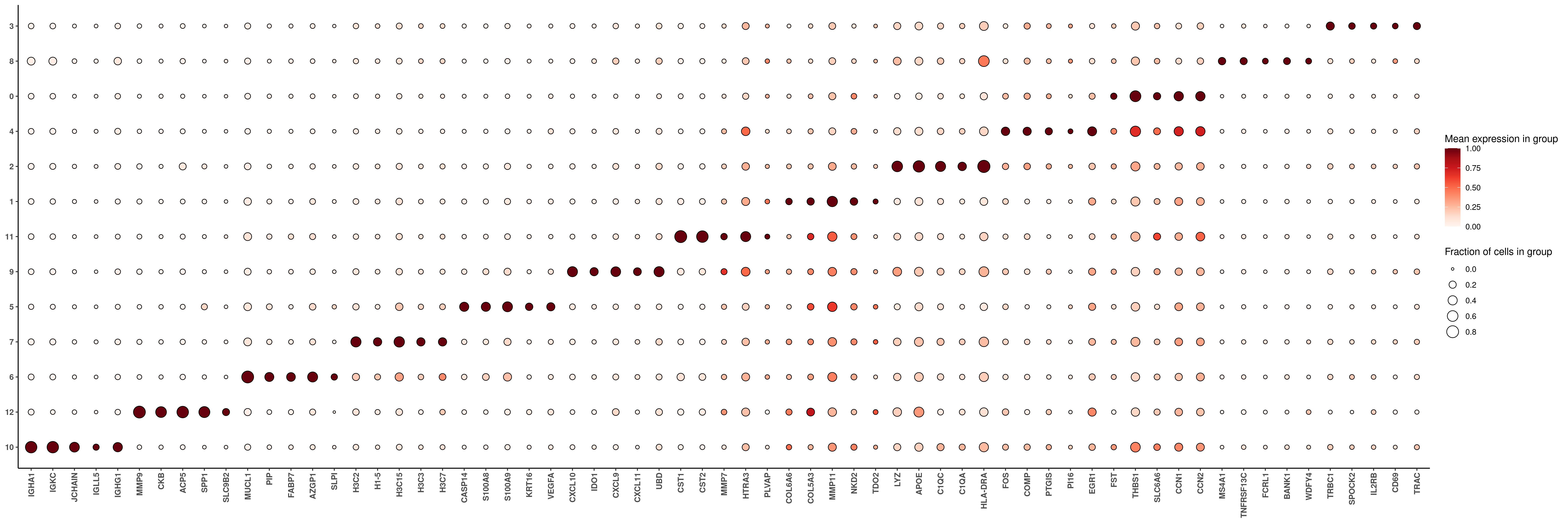
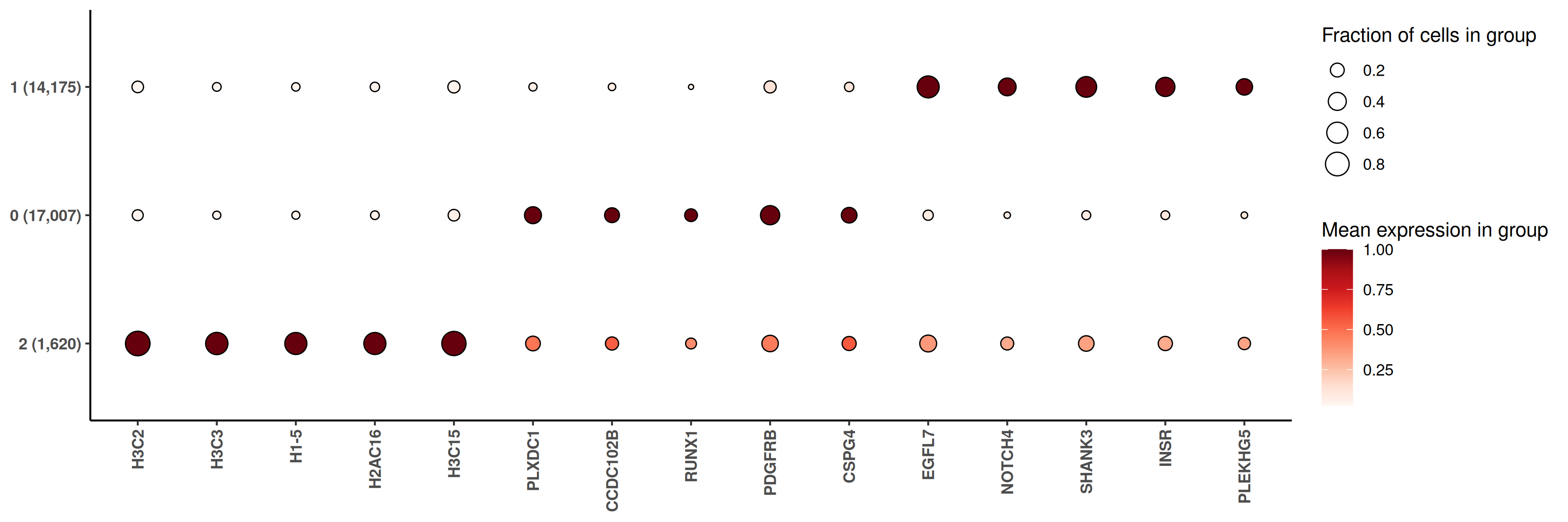
Based on the markers present, we can see that there are multiple non-fibroblast cell subtypes contained within this cluster. We name the fibroblast subtypes and note the immune subtypes to put into the immune-focused hieratype subtyping.
Cell type
Evaluation
Name
0
Key markers CCN1, CCN2
Myofibroblasts
1
Key markers COL6A6, MMP11
Matrix fibroblasts
2
APC markers HLA-DRA, C1QC
Immune subtype
3
T cell markers TRBC1, IL2RB
Immune subtype
4
Key markers FOS, PTGIS, EGR1
iCAFs
5
Inflammatory markers S100A8/A9
Immune subtype
6
Metabolic markers MUCL1, PIP, FABP7, unclear where to put these. Choosing based on XY and UMAP localization.
Immune subtype
7
Proliferation markers histones. Choosing based on UMAP proximity.
Immune subtype
8
B cell markers MS4A1, BANK1
Immune subtype
9
Key markers CXCL10, IDO1
Interferon-activated CAFs
10
Plasma markers IGHA1, IGKC, JCHAIN
Immune subtype
11
Markers CST1/2, MMP7, unclear. Choosing based on UMAP localization.
Immune subtype
12
Immune markers MMP9, SPP1
Immune subtype
Add cell type names to fibroblast subtypes.
Show the code
# Follows table above. Any that are not fibroblasts will be listed as NAfibro_assignments <-readRDS(file =paste0(celltyping_dir, "/Data/fibro_cluster_assignments.rds"))fibro_assignments$minor_cell_type <-NAfibro_assignments$minor_cell_type[which(fibro_assignments$seurat_clusters ==0)] <-"Myofibroblasts"fibro_assignments$minor_cell_type[which(fibro_assignments$seurat_clusters ==1)] <-"Matrix fibroblasts"fibro_assignments$minor_cell_type[which(fibro_assignments$seurat_clusters ==4)] <-"Inflammatory CAFs"fibro_assignments$minor_cell_type[which(fibro_assignments$seurat_clusters ==9)] <-"Interferon-activated CAFs"saveRDS(fibro_assignments, file =paste0(celltyping_dir, "/Data/fibro_cluster_assignments.rds"))
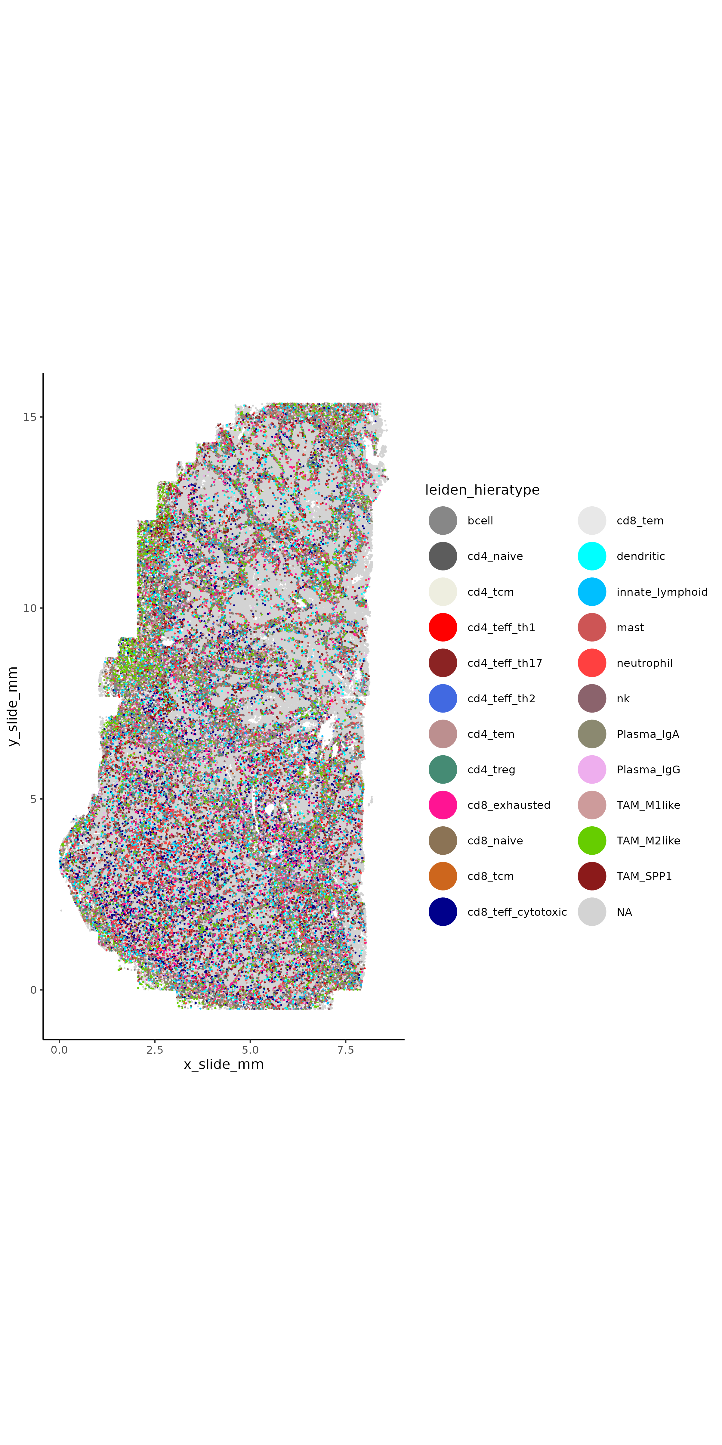
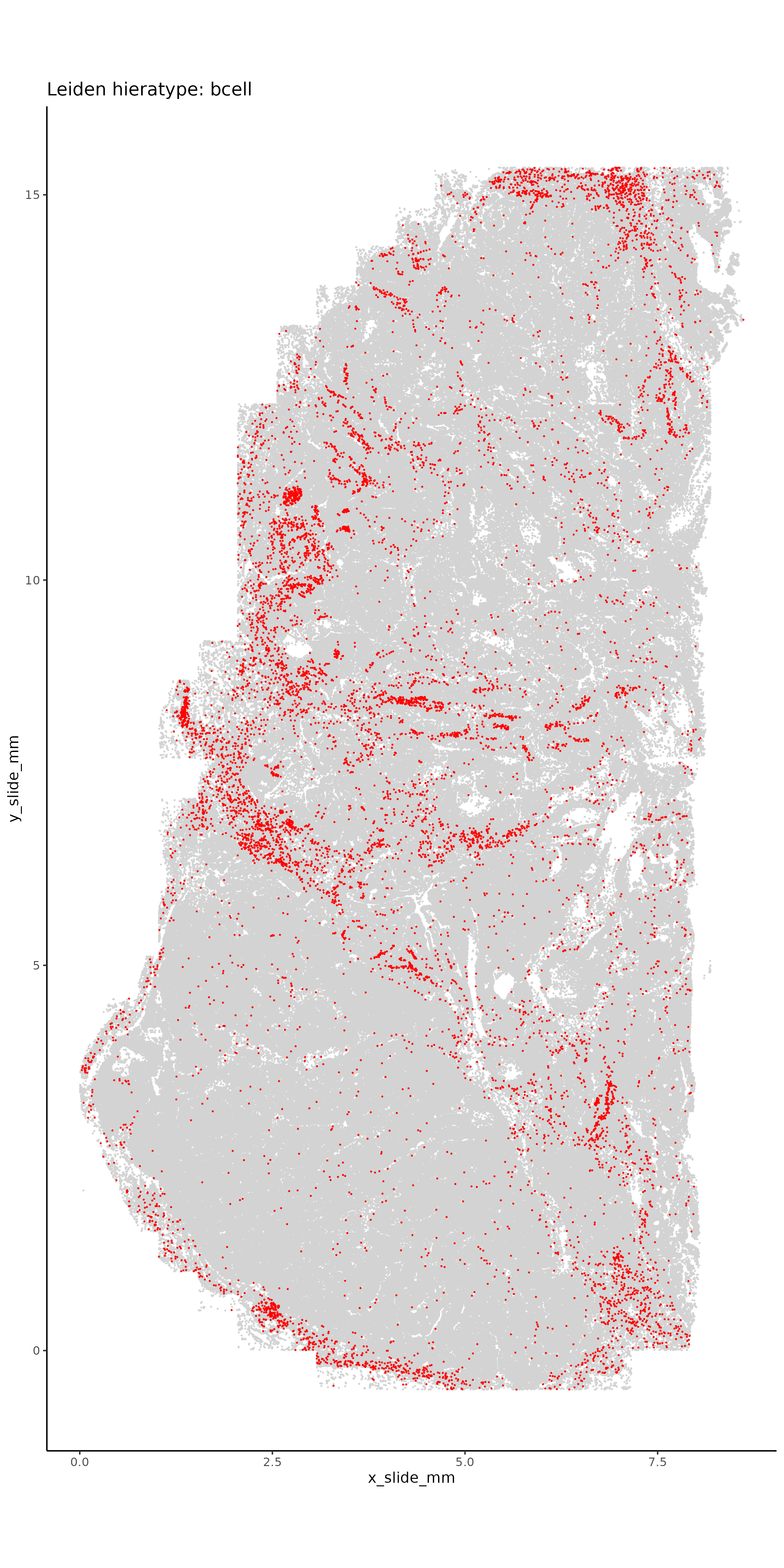
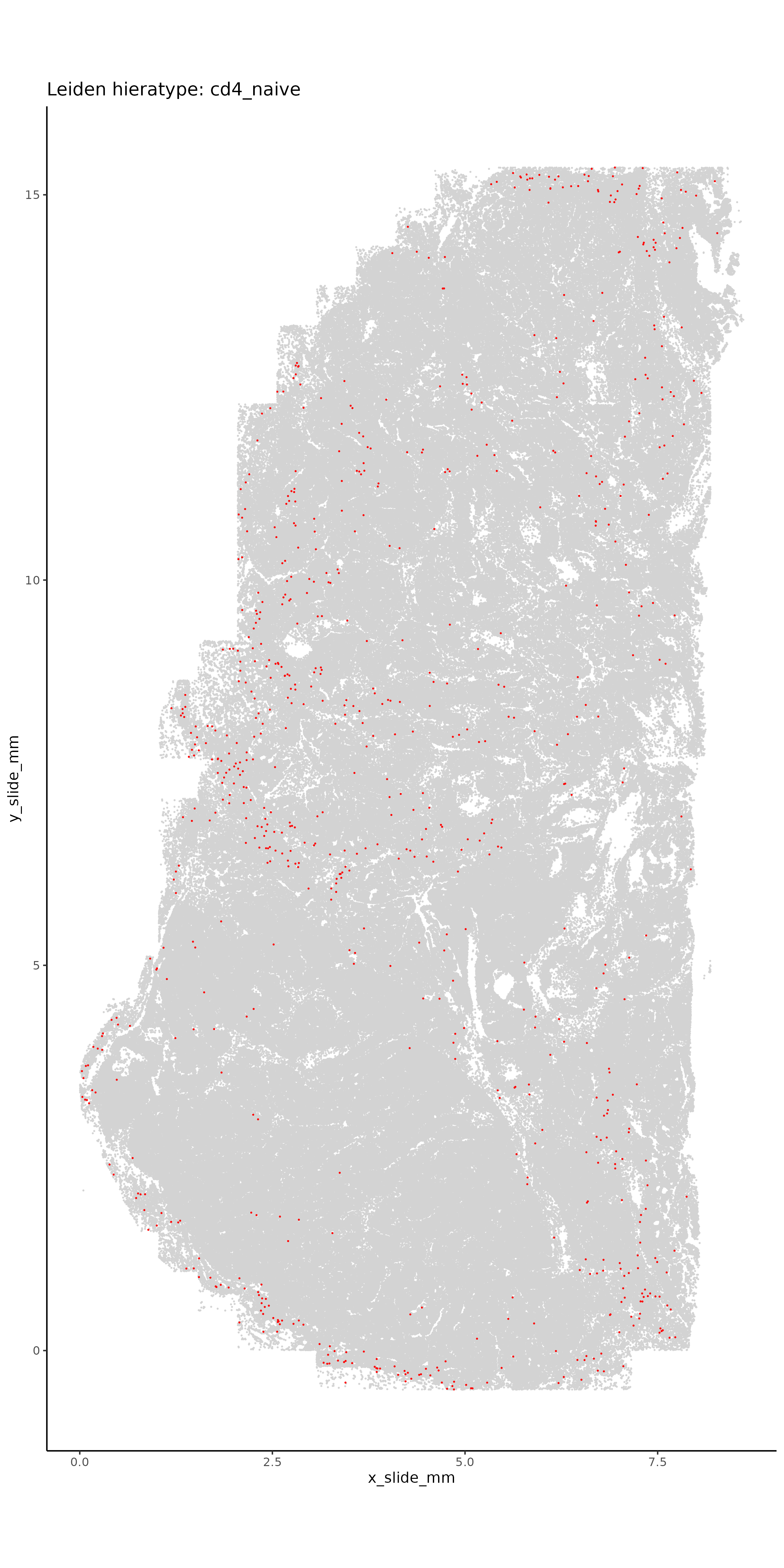
To better assign the immune cells, we use HieraType, a marker-based approach to assigning cell types. We start with marker-based gene lists included in the HieraType package and add in some additional cell subtypes that we expect to be present in this dataset. As described in the table above, we’ll use unsupervised clusters 3, 6, 15, and 16 for this immune classification as well as some of the fibroblast subclusters.
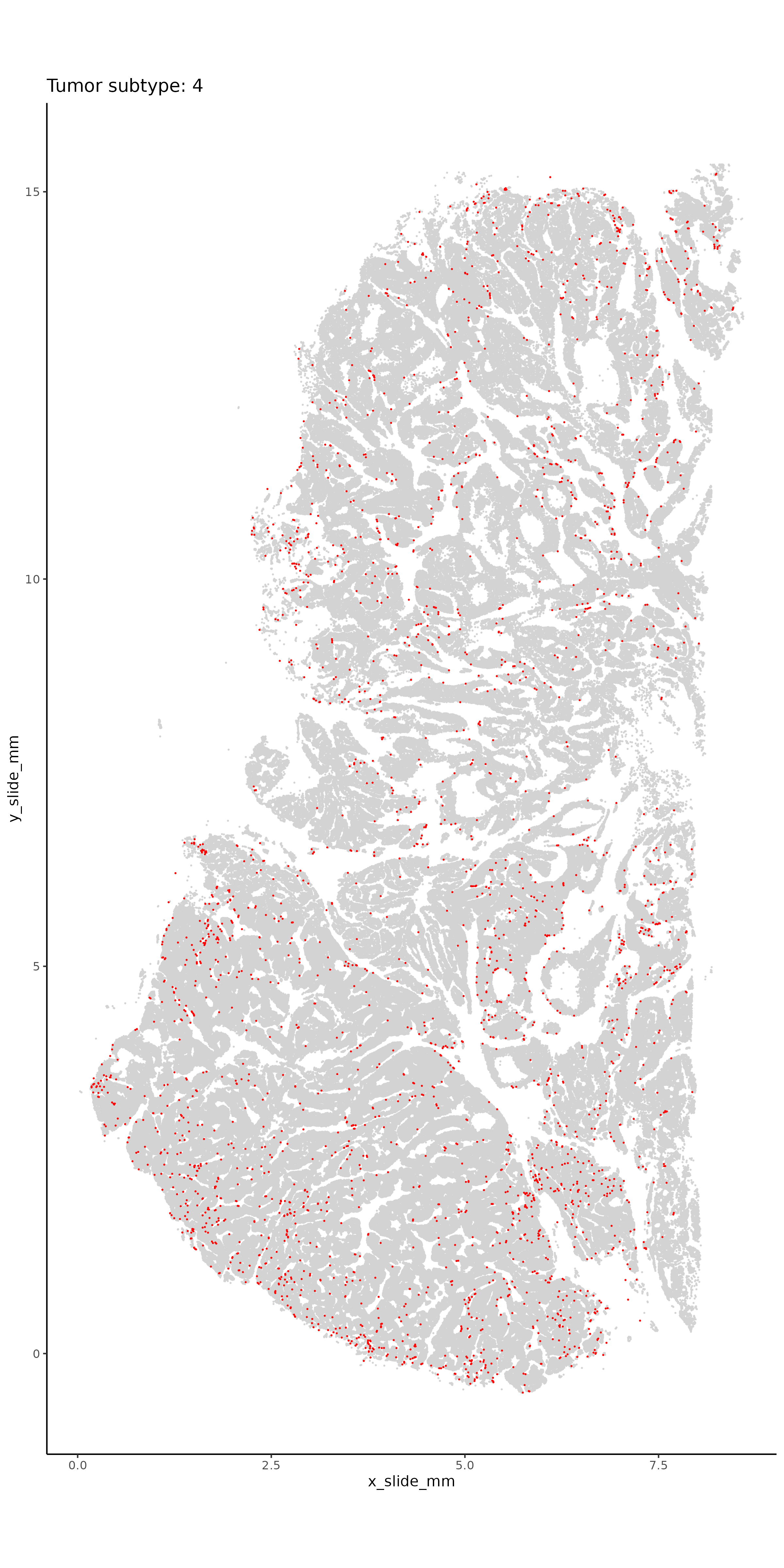
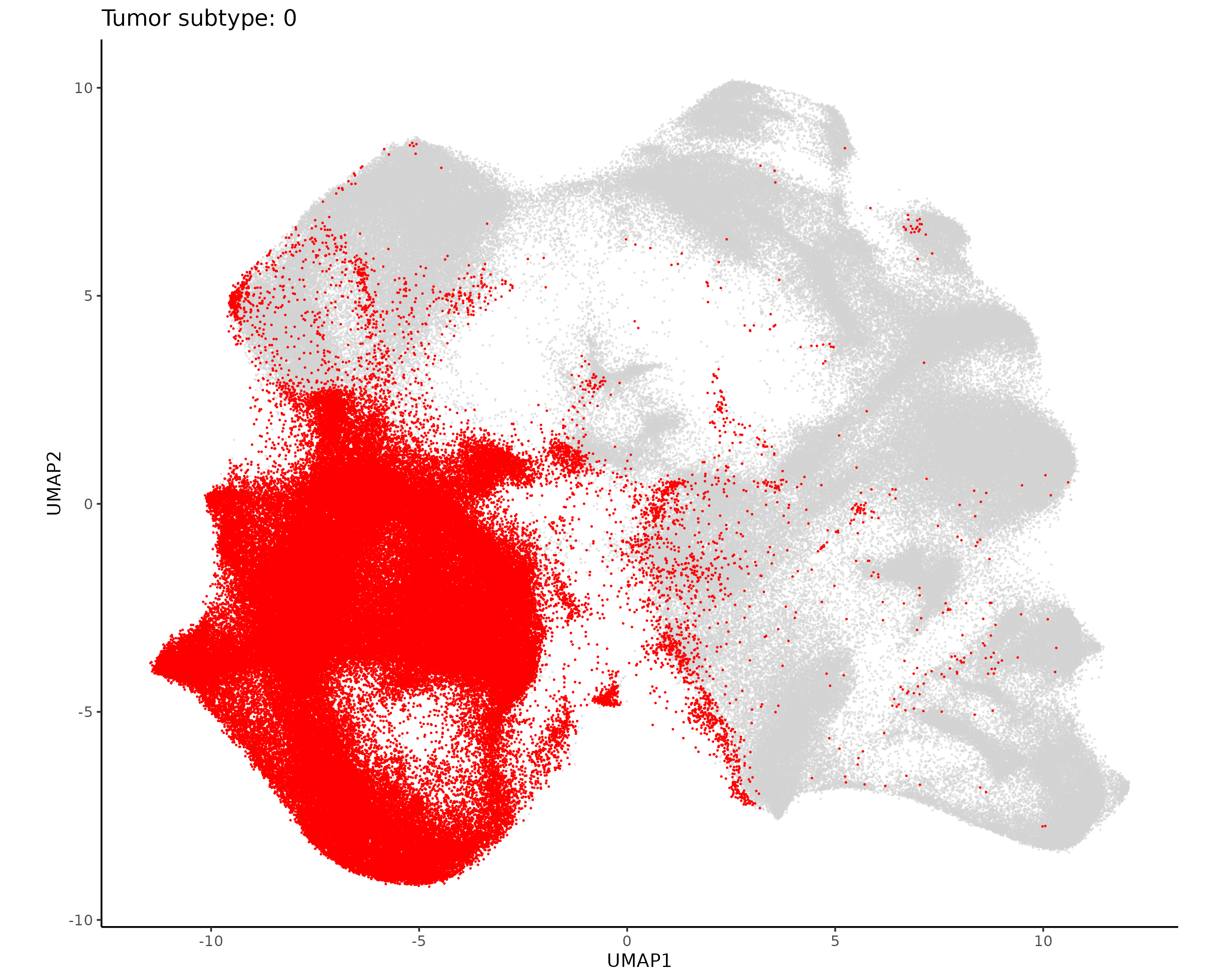
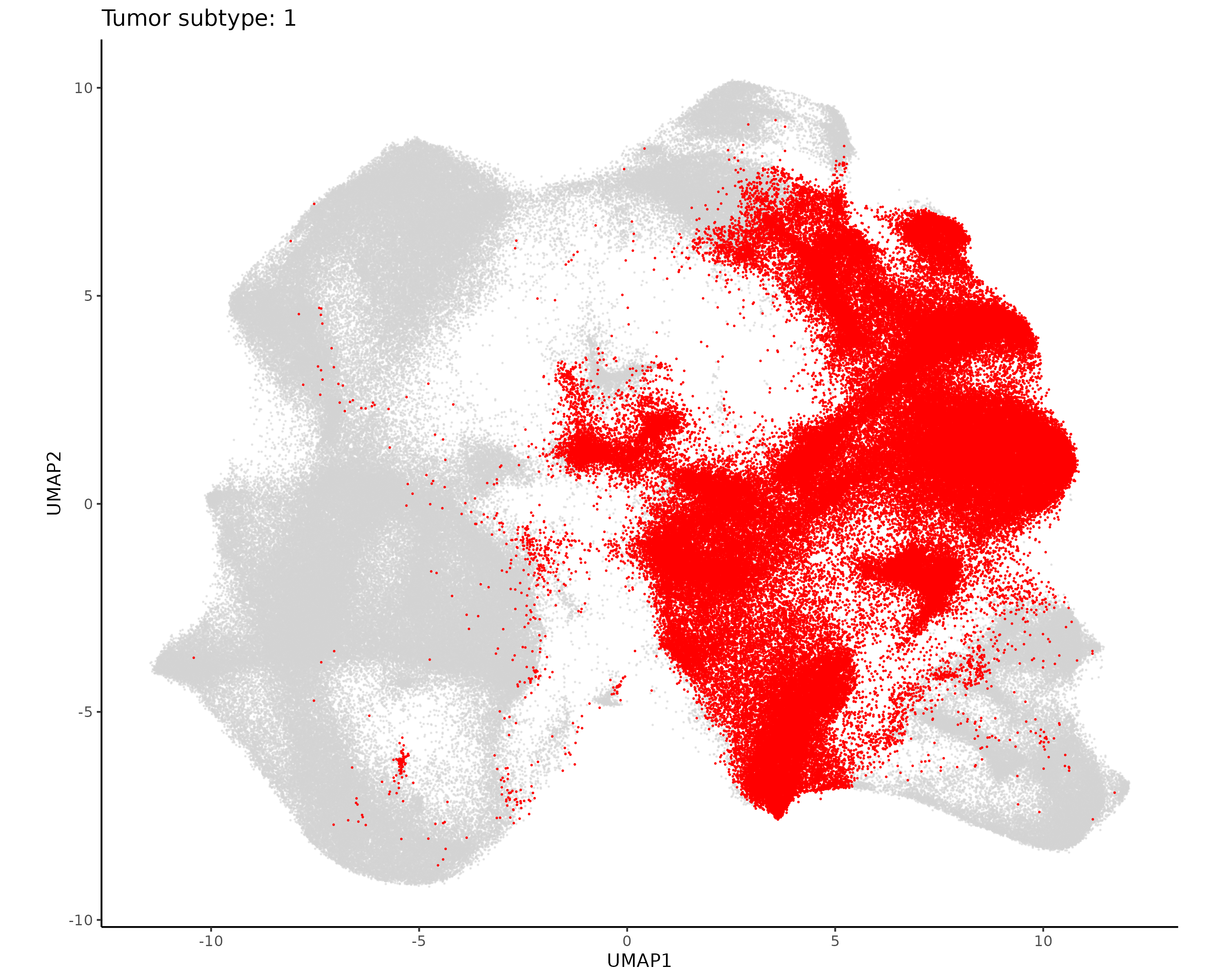
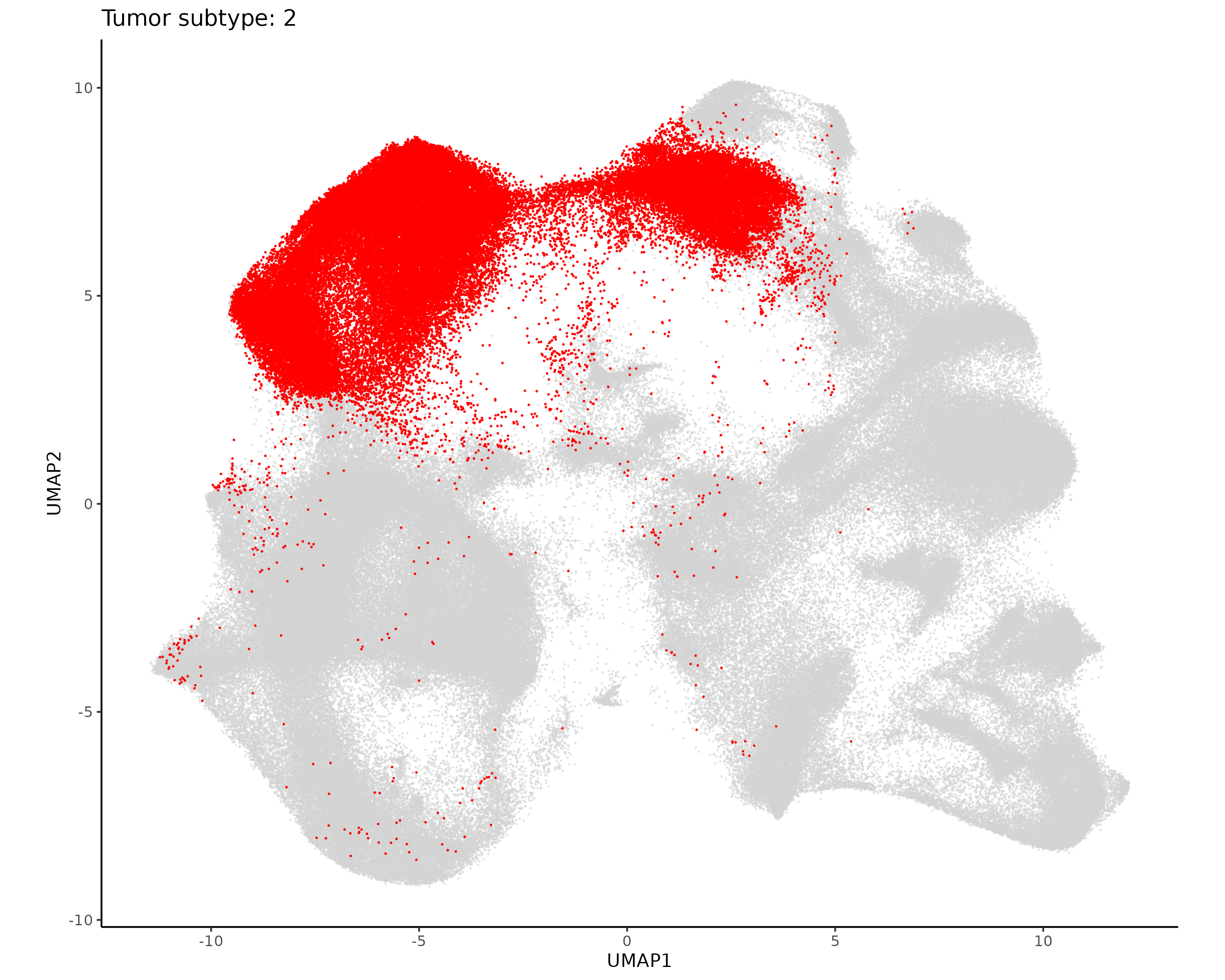
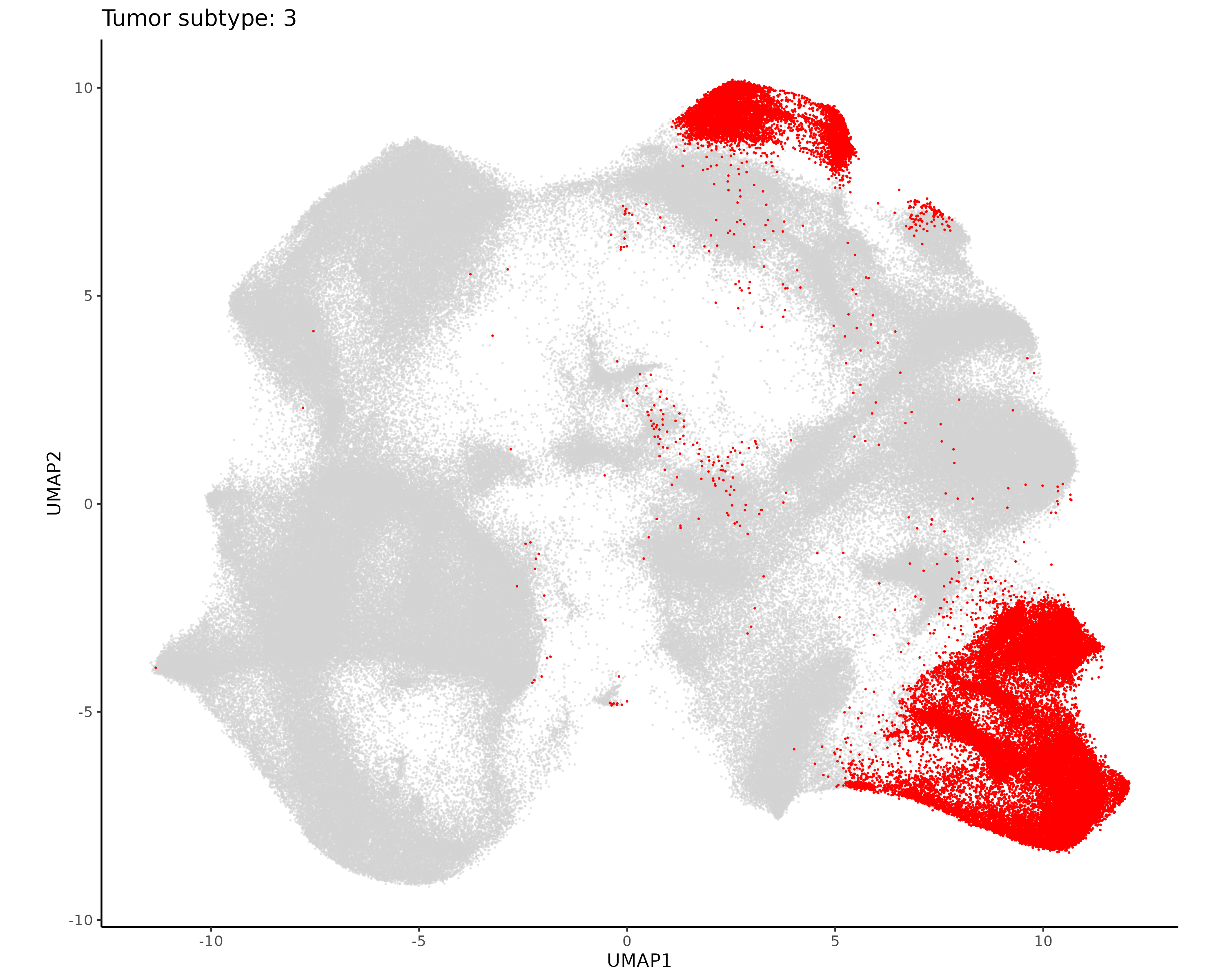
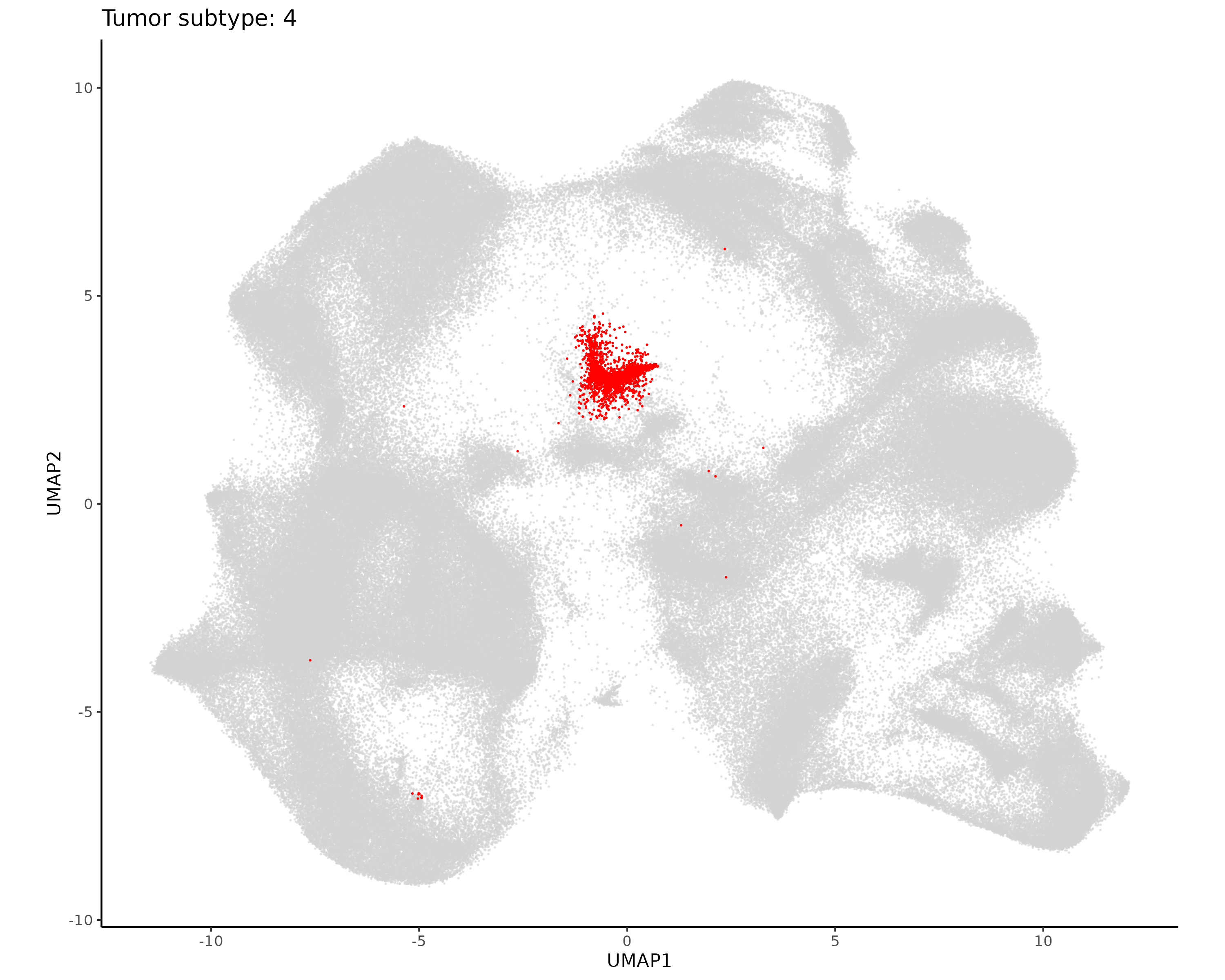
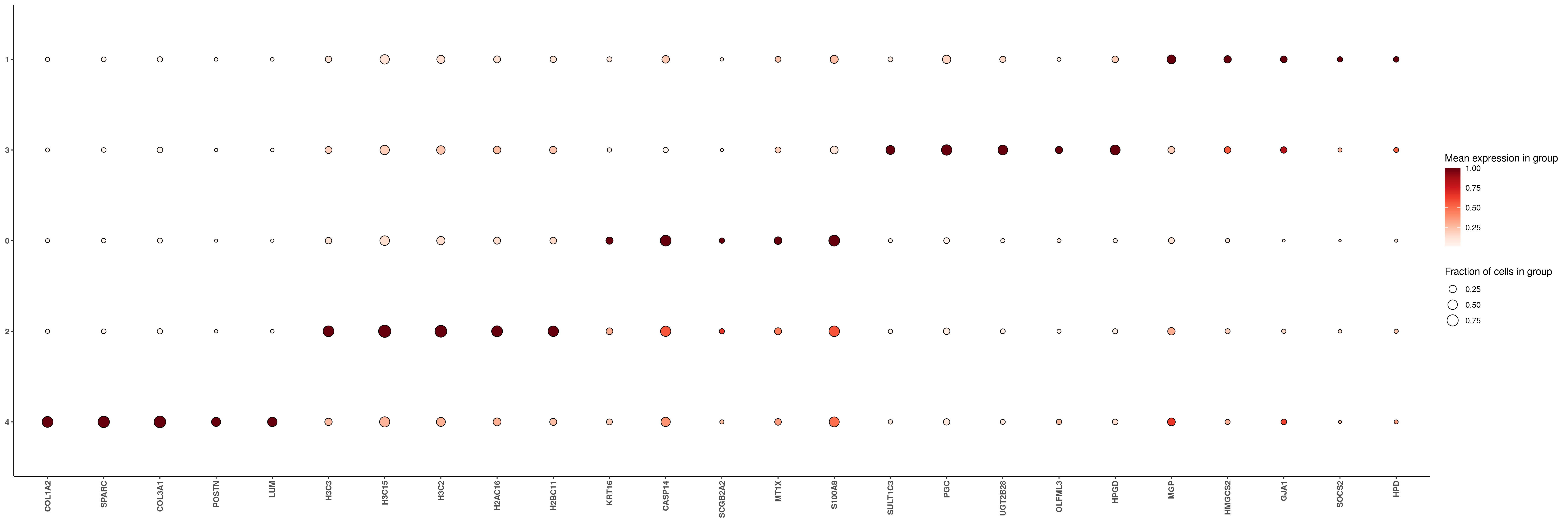
The initial unsupervised clustering had more tumor subclusters than we’ll use in this analysis. Here we take all the tumor cells, repeat initial preprocessing so that highly variable genes are chosen based on the tumor cells, and use Leiden clustering with low resolution to separate the tumor cells into about five major clusters.
Show the code
if (!("seu.obj"%in%ls())){ seu.obj <-readRDS(results_list$seurat_file_postLeiden)}# Subset the seurat object to only include tumor cellstumor_leiden <-c(0, 1, 4, 5, 7, 8, 10, 12:14)tumor_idx <-which(seu.obj@meta.data$seurat_clusters %in% tumor_leiden)seu.tumor <- seu.obj[,tumor_idx]# Repeat preprocessing, dimension reduction, and leiden clusteringseu.tumor <-NormalizeData(seu.tumor, normalization.method ="RC", scale.factor =mean(seu.tumor@meta.data$nCount_RNA))seu.tumor <-FindVariableFeatures(seu.tumor, selection.method ="vst", nfeatures =3000)seu.tumor <-ScaleData(seu.tumor)seu.tumor <-RunPCA(seu.tumor, features =VariableFeatures(seu.tumor))umapobj <-make_umap(seu.tumor@reductions$pca@cell.embeddings)seu.tumor[["umap"]] <- umapobj$umpseu.tumor[["umapgrph"]] <- Seurat::as.Graph(umapobj$grph)seu.tumor <- Seurat::FindClusters(seu.tumor, graph.name ="umapgrph", resolution =0.2)# Save this Seurat object and assignments to filessaveRDS(seu.tumor, file =paste0(objects_dir, "/seurat_tumor_obj.rds"))tumor_assignments <- seu.tumor@meta.data[,c("cell_ID", "seurat_clusters")]saveRDS(tumor_assignments, file =paste0(celltyping_dir, "/Data/tumor_cluster_assignments.rds"))
Plot tumor subclusters for evaluation.
Show the code
# Plot it in XY space with random colorsset.seed(2025)my_pal <-sample(colors(distinct =TRUE), length(unique(seu.tumor@meta.data$seurat_clusters)))names(my_pal) <-unique(seu.tumor@meta.data$seurat_clusters)ggplot(seu.tumor@meta.data,aes(x = x_slide_mm, y = y_slide_mm, color =as.factor(seurat_clusters))) +geom_point(size =0.1) +scale_color_manual(values = my_pal, na.value ="lightgrey") +theme_classic() +coord_fixed() +guides(colour =guide_legend(override.aes =list(size=10)))ggsave(filename =paste0(dimRed_dir, "/Plots/XY_tumor_subclusters.png"),width =8, height =16, units ="in")# Plot each cell type separatelyfor (ct inunique(seu.tumor@meta.data$seurat_clusters)){if(is.na(ct)){next}ggplot(seu.tumor@meta.data,aes(x = x_slide_mm, y = y_slide_mm)) +geom_point(size =0.05, color ="lightgrey") +geom_point(data = seu.tumor@meta.data %>%filter(seurat_clusters == ct),aes(x = x_slide_mm, y = y_slide_mm),size =0.05, color ="red") +theme_classic() +coord_fixed() +ggtitle(paste0("Tumor subtype: ", ct))ggsave(filename =paste0(dimRed_dir, "/Plots/XY_tumor_subtype_", ct, ".png"),width =8, height =16, units ="in")}# Plot it in UMAP spaceDimPlot(seu.tumor, group.by ="seurat_clusters", reduction ="umap", label = T) +scale_color_manual(values = my_pal, na.value ="lightgrey") +coord_fixed()ggsave(filename =paste0(dimRed_dir, "/Plots/umap_tumor_subtype.png"),width =16, height =12, units ="in")# Plot each cell type separately in UMAP spaceplot.df <- seu.tumor@meta.dataplot.df$UMAP1 <- seu.tumor@reductions$umap@cell.embeddings[,1]plot.df$UMAP2 <- seu.tumor@reductions$umap@cell.embeddings[,2]for (ct inunique(plot.df$seurat_clusters)){ggplot(plot.df,aes(x = UMAP1, y = UMAP2)) +geom_point(size =0.05, alpha =0.5, color ="lightgrey") +geom_point(data = plot.df %>%filter(seurat_clusters == ct),aes(x = UMAP1, y = UMAP2),size =0.05, color ="red") +theme_classic() +coord_fixed() +ggtitle(paste0("Tumor subtype: ", ct))ggsave(filename =paste0(dimRed_dir, "/Plots/UMAP_tumor_subtype_", ct, ".png"),width =10, height =8, units ="in")}# Marker heatmap## prepare data for marker gene heatmap:fc_subclus_ctl_gran <-clusterwise_foldchange_metrics(seu.tumor[["RNA"]]@counts ,metadata = seu.tumor@meta.data ,cluster_column ="seurat_clusters")# subtract background from the mean per-cluster expression profiles:neg_counts_tumor = seu.tumor@assays$negprobes$countsfor (name inunique(seu.tumor@meta.data$seurat_clusters)) {if(is.na(name)){next} isthiscelltype <- seu.tumor@meta.data$seurat_clusters == name meannegthiscelltype <- Matrix::mean(neg_counts_tumor[, isthiscelltype]) fc_subclus_ctl_gran$cluster_expr[fc_subclus_ctl_gran$cluster == name] <-pmax(fc_subclus_ctl_gran$cluster_expr[fc_subclus_ctl_gran$cluster == name] - meannegthiscelltype, 0)}# create the heatmap:hm_lh <-add_ncells(marker_heatmap(fc_subclus_ctl_gran))png(filename =paste0(dimRed_dir, "/Plots/heatmap_tumor_subcluster_negRemoved.png"),width =24, height =8, units ="in", res =300)print(hm_lh)dev.off()# Save results fileresults_list$tumor_subcluster_color_pal <- my_palsaveRDS(results_list, results_list_file)
The initial Leiden clustering had only one vasculature cluster, but from previous experience with this sample we expect that we should be able to identify pericytes and endothelial cells separately. Here we take the vasculature cells, repeat initial preprocessing so that highly variable genes are chosen based on these cells, and use unsupervised clustering to separate these cells into two or three clusters.
Show the code
if (!("seu.obj"%in%ls())){ seu.obj <-readRDS(results_list$seurat_file_postLeiden)}# Subset the seurat object to only include tumor cellsvasc_leiden <-c(9)vasc_idx <-which(seu.obj@meta.data$seurat_clusters %in% vasc_leiden)seu.vasc <- seu.obj[,vasc_idx]# Repeat preprocessing, dimension reduction, and leiden clusteringseu.vasc <-NormalizeData(seu.vasc, normalization.method ="RC", scale.factor =mean(seu.vasc@meta.data$nCount_RNA))seu.vasc <-FindVariableFeatures(seu.vasc, selection.method ="vst", nfeatures =3000)seu.vasc <-ScaleData(seu.vasc)seu.vasc <-RunPCA(seu.vasc, features =VariableFeatures(seu.vasc))umapobj <-make_umap(seu.vasc@reductions$pca@cell.embeddings)seu.vasc[["umap"]] <- umapobj$umpseu.vasc[["umapgrph"]] <- Seurat::as.Graph(umapobj$grph)seu.vasc <- Seurat::FindClusters(seu.vasc, graph.name ="umapgrph", resolution =0.1)# Save this Seurat object and assignments to filessaveRDS(seu.vasc, file =paste0(objects_dir, "/seurat_vasc_obj.rds"))vasc_assignments <- seu.vasc@meta.data[,c("cell_ID", "seurat_clusters")]saveRDS(vasc_assignments, file =paste0(celltyping_dir, "/Data/vasc_cluster_assignments.rds"))# Save a few quick plots for evaluation# Plot it in XY space with random colorsset.seed(2025)my_pal <-sample(colors(distinct =TRUE), length(unique(seu.vasc@meta.data$seurat_clusters)))names(my_pal) <-unique(seu.vasc@meta.data$seurat_clusters)ggplot(seu.vasc@meta.data,aes(x = x_slide_mm, y = y_slide_mm, color =as.factor(seurat_clusters))) +geom_point(size =0.01) +scale_color_manual(values = my_pal, na.value ="lightgrey") +theme_classic() +coord_fixed() +guides(colour =guide_legend(override.aes =list(size=10)))ggsave(filename =paste0(celltyping_dir, "/Plots/XY_vasculature_subclusters.png"),width =8, height =16, units ="in")# Plot each cell type separatelyfor (ct inunique(seu.vasc@meta.data$seurat_clusters)){if(is.na(ct)){next}ggplot(seu.vasc@meta.data,aes(x = x_slide_mm, y = y_slide_mm)) +geom_point(size =0.05, color ="lightgrey") +geom_point(data = seu.vasc@meta.data %>%filter(seurat_clusters == ct),aes(x = x_slide_mm, y = y_slide_mm),size =0.05, color ="red") +theme_classic() +coord_fixed() +ggtitle(paste0("Vascular subtype: ", ct))ggsave(filename =paste0(celltyping_dir, "/Plots/XY_vasculature_subtype_", ct, ".png"),width =8, height =16, units ="in")}# UMAPDimPlot(seu.vasc) +coord_fixed()ggsave(file =paste0(celltyping_dir, "/Plots/UMAP_vasculature.png"))# Marker heatmap## prepare data for marker gene heatmap:fc_subclus_ctl_gran <-clusterwise_foldchange_metrics(seu.vasc[["RNA"]]@counts ,metadata = seu.vasc@meta.data ,cluster_column ="seurat_clusters")# subtract background from the mean per-cluster expression profiles:neg_counts_vasc = seu.vasc@assays$negprobes$countsfor (name inunique(seu.vasc@meta.data$seurat_clusters)) {if(is.na(name)){next} isthiscelltype <- seu.vasc@meta.data$seurat_clusters == name meannegthiscelltype <- Matrix::mean(neg_counts_vasc[, isthiscelltype]) fc_subclus_ctl_gran$cluster_expr[fc_subclus_ctl_gran$cluster == name] <-pmax(fc_subclus_ctl_gran$cluster_expr[fc_subclus_ctl_gran$cluster == name] - meannegthiscelltype, 0)}# create the heatmap:hm_lh <-add_ncells(marker_heatmap(fc_subclus_ctl_gran))png(filename =paste0(celltyping_dir, "/Plots/heatmap_vasculature_subcluster_negRemoved.png"),width =12, height =4, units ="in", res =300)print(hm_lh)dev.off()
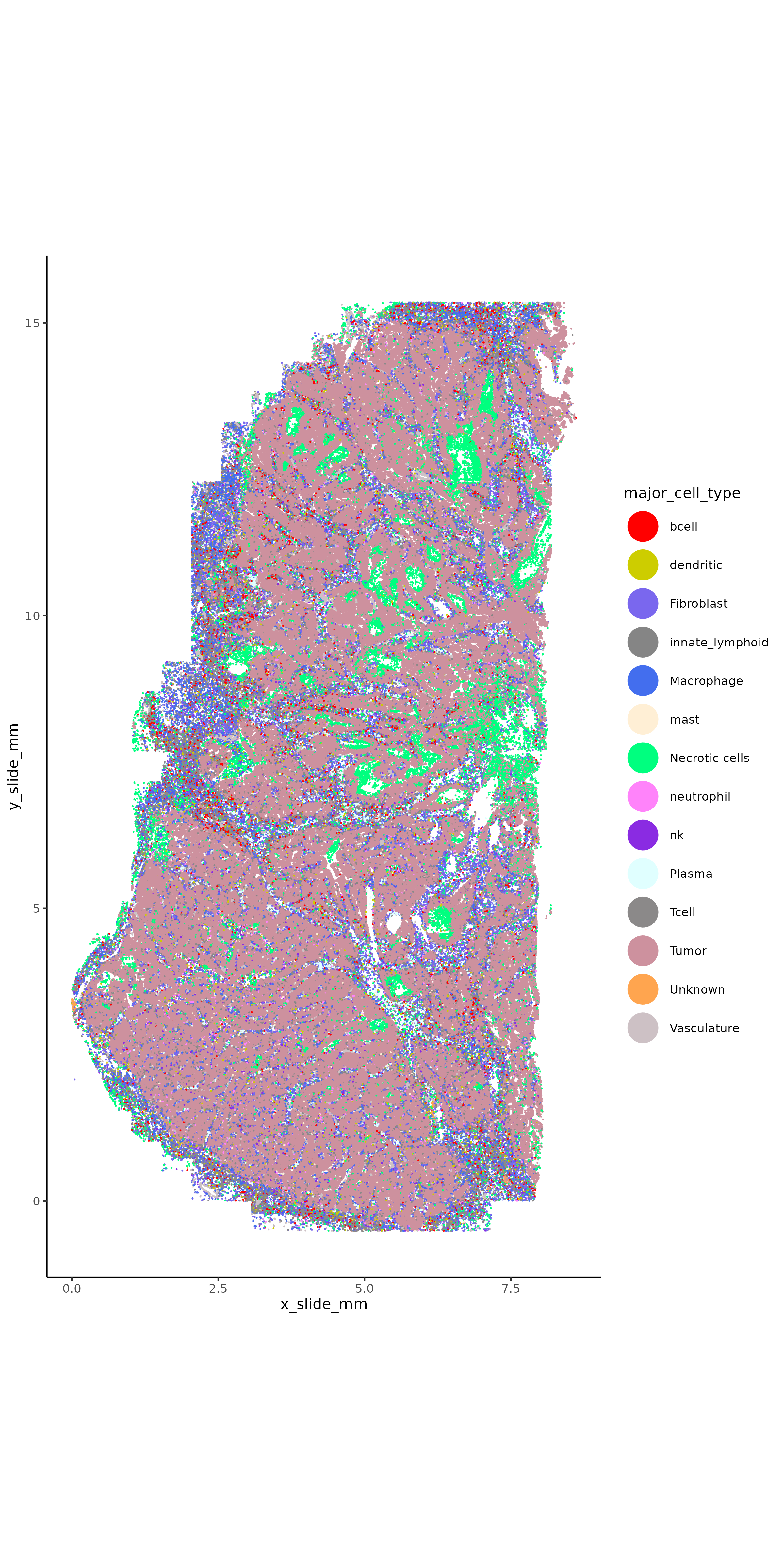
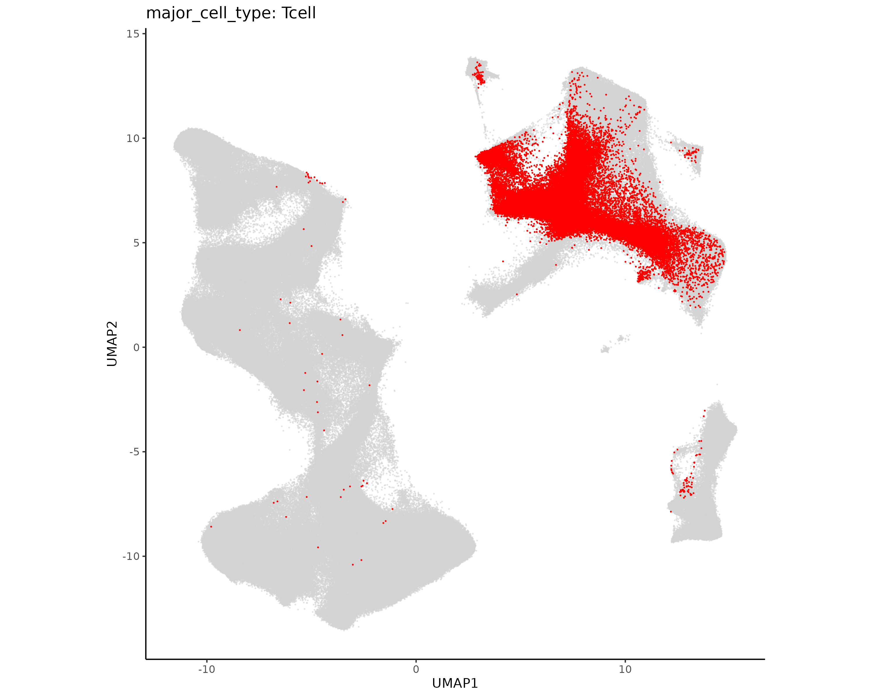
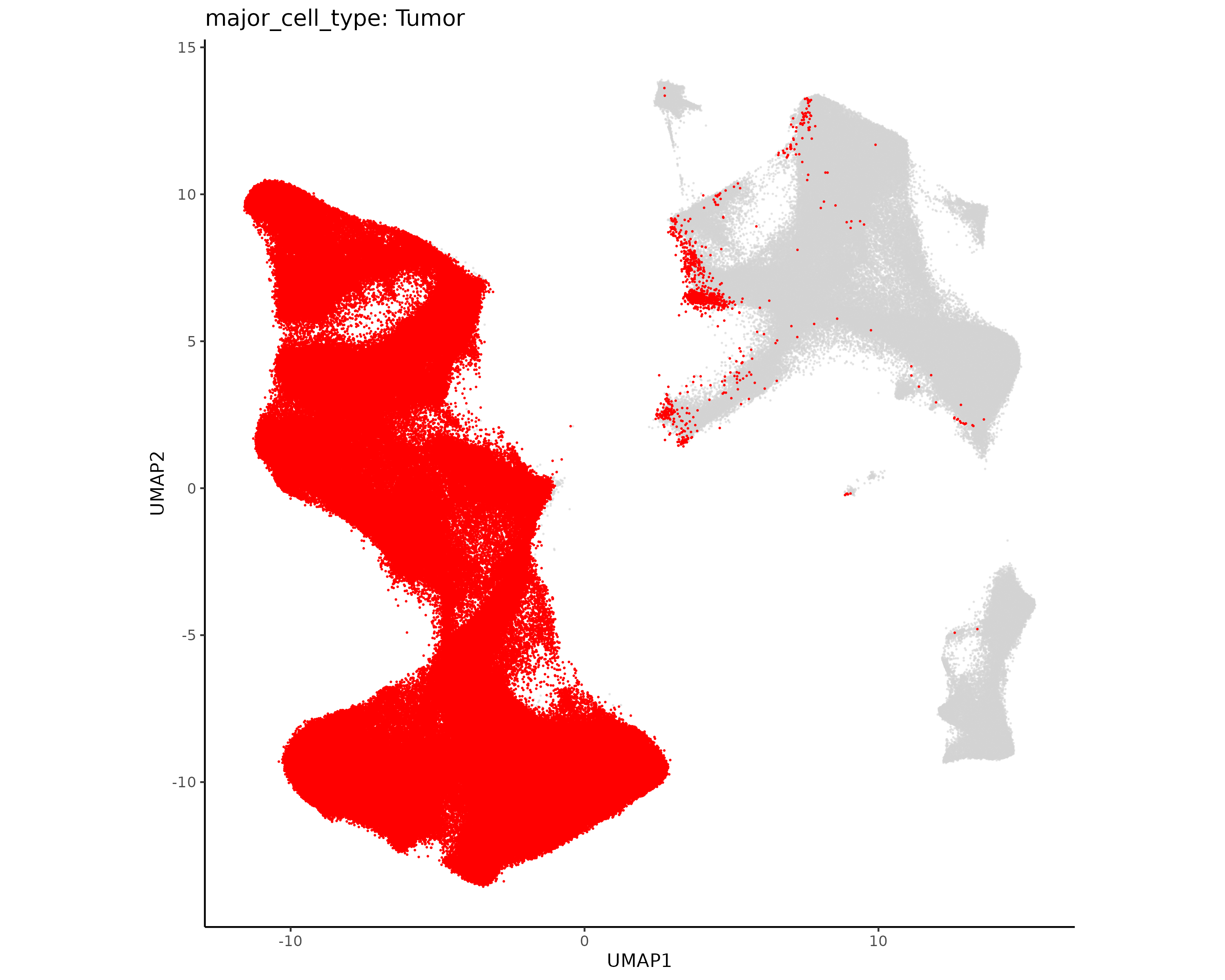
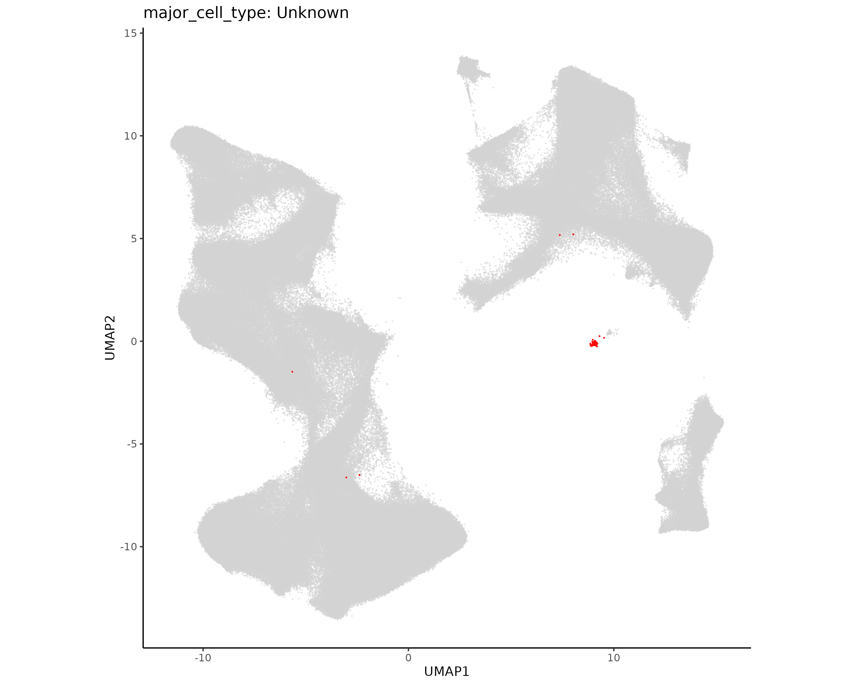
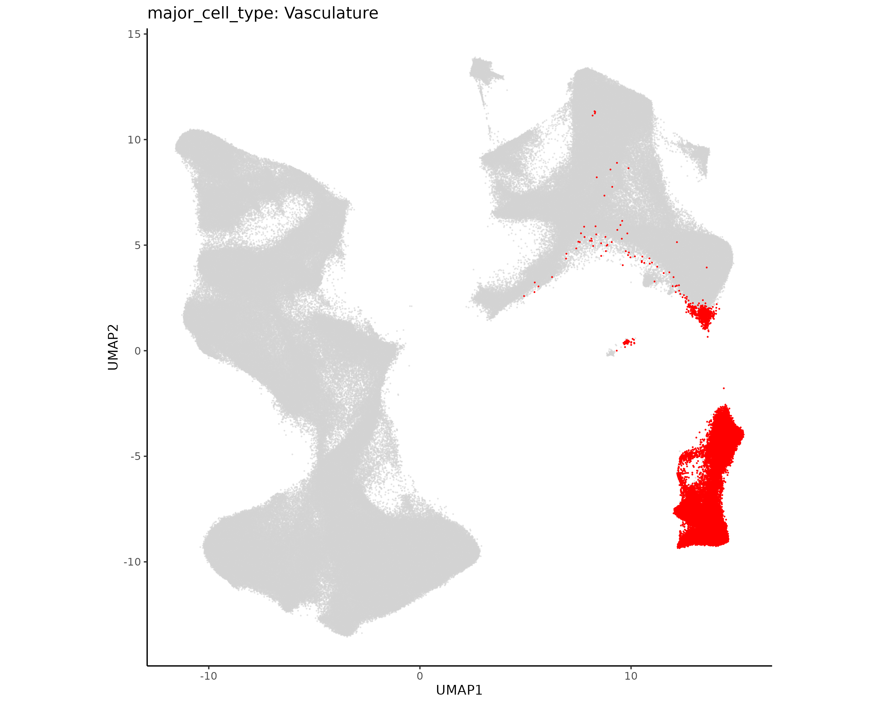
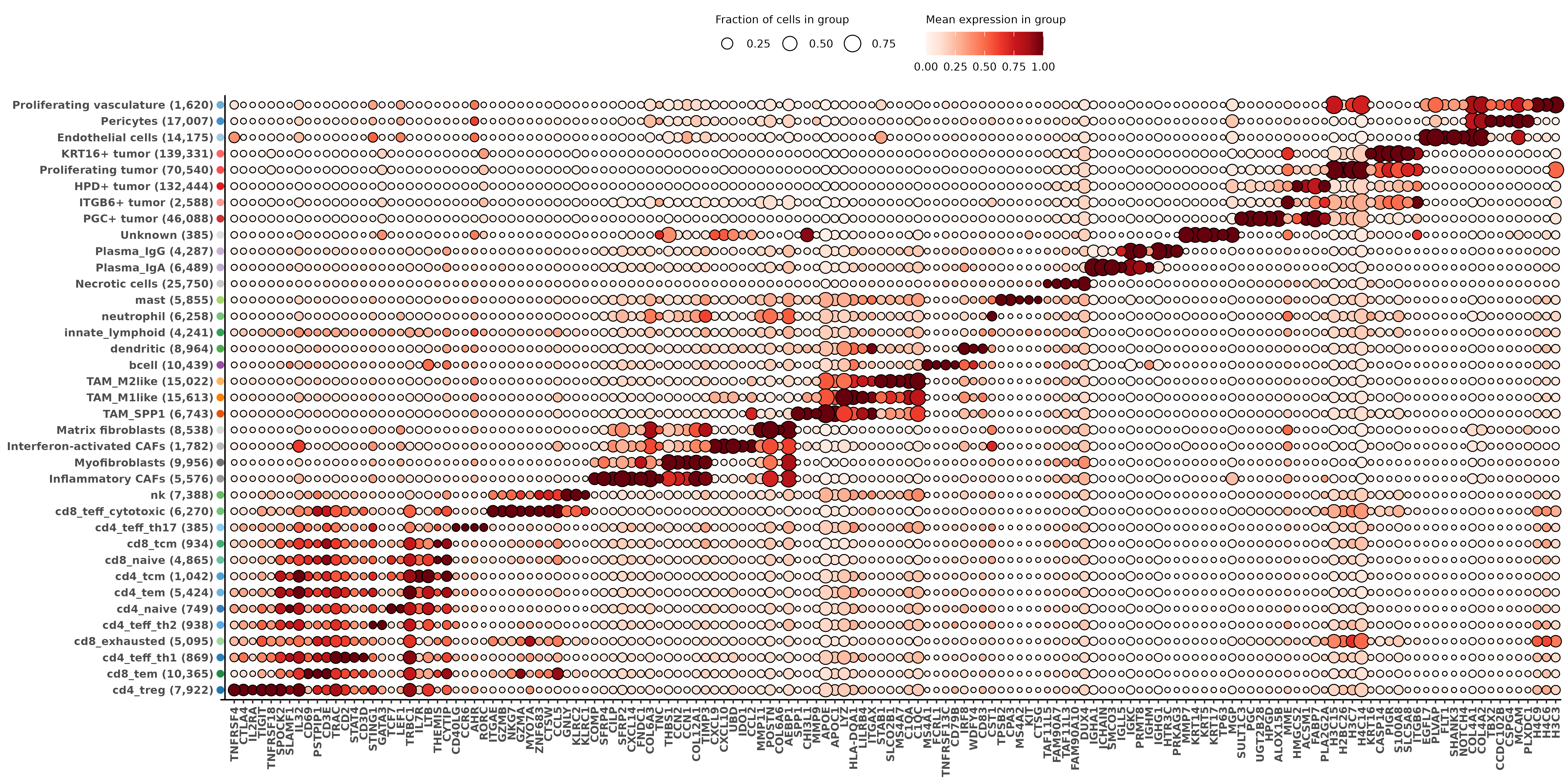
Here we join all the above annotations into the full Seurat object. We make two cell typing columns - one shows major cell types (tumor, T cell, etc) and the second shows the finer minor cell subtypes. We also make standard plots to show each of these.
Show the code
if (!("seu.obj"%in%ls())){ seu.obj <-readRDS(results_list$seurat_file_postLeiden)}# Read in cell subtyping resultsfibro_assignments <-readRDS(file =paste0(celltyping_dir, "/Data/fibro_cluster_assignments.rds"))immune_typing <-readRDS(file =paste0(dimRed_dir, "/Data/immune_hieratype_res.rds"))tumor_assignments <-readRDS(file =paste0(celltyping_dir, "/Data/tumor_cluster_assignments.rds"))vasc_assignments <-readRDS(file =paste0(celltyping_dir, "/Data/vasc_cluster_assignments.rds"))# Extract immune typing assignments to same format as other subtypingsimmune_assignments <-as.data.frame(immune_typing$post_probs$l1)row.names(immune_assignments) <- immune_assignments$cell_ID# Add fine subtypes to seurat objectseu.obj@meta.data$minor_cell_type <-NAseu.obj@meta.data[fibro_assignments$cell_ID, "minor_cell_type"] <- fibro_assignments$minor_cell_typeseu.obj@meta.data[tumor_assignments$cell_ID, "minor_cell_type"] <- tumor_assignments$minor_cell_typeseu.obj@meta.data[vasc_assignments$cell_ID, "minor_cell_type"] <- vasc_assignments$minor_cell_typeseu.obj@meta.data[immune_assignments$cell_ID, "minor_cell_type"] <- immune_assignments$celltype_granular# Two clusters that did not get subtypedseu.obj@meta.data$minor_cell_type[which(seu.obj@meta.data$seurat_clusters ==11)] <-"Necrotic cells"seu.obj@meta.data$minor_cell_type[which(seu.obj@meta.data$seurat_clusters ==17)] <-"Unknown"# Add major typesseu.obj@meta.data$major_cell_type <- seu.obj@meta.data$minor_cell_typeseu.obj@meta.data$major_cell_type <- dplyr::recode(seu.obj@meta.data$major_cell_type,"cd4_naive"="Tcell","cd4_tcm"="Tcell","cd4_teff_th1"="Tcell","cd4_teff_th2"="Tcell","cd4_teff_th17"="Tcell","cd4_tem"="Tcell","cd4_treg"="Tcell","cd8_exhausted"="Tcell","cd8_naive"="Tcell","cd8_tcm"="Tcell","cd8_teff_cytotoxic"="Tcell","cd8_tem"="Tcell","Endothelial cells"="Vasculature","HPD+ tumor"="Tumor","Inflammatory CAFs"="Fibroblast","Interferon-activated CAFs"="Fibroblast","KRT16+ tumor"="Tumor","ITGB6+ tumor"="Tumor","Matrix fibroblasts"="Fibroblast","Myofibroblasts"="Fibroblast","Pericytes"="Vasculature","PGC+ tumor"="Tumor","Plasma_IgA"="Plasma","Plasma_IgG"="Plasma","Proliferating tumor"="Tumor","Proliferating vasculature"="Vasculature","TAM_M1like"="Macrophage","TAM_M2like"="Macrophage","TAM_SPP1"="Macrophage")# Save seurat object with cell typesresults_list$seurat_file_postCellTyping <-paste0(objects_dir, "/seurat_object_postCellTyping.rds")saveRDS(results_list, results_list_file)saveRDS(seu.obj, results_list$seurat_file_postCellTyping)
Show the code
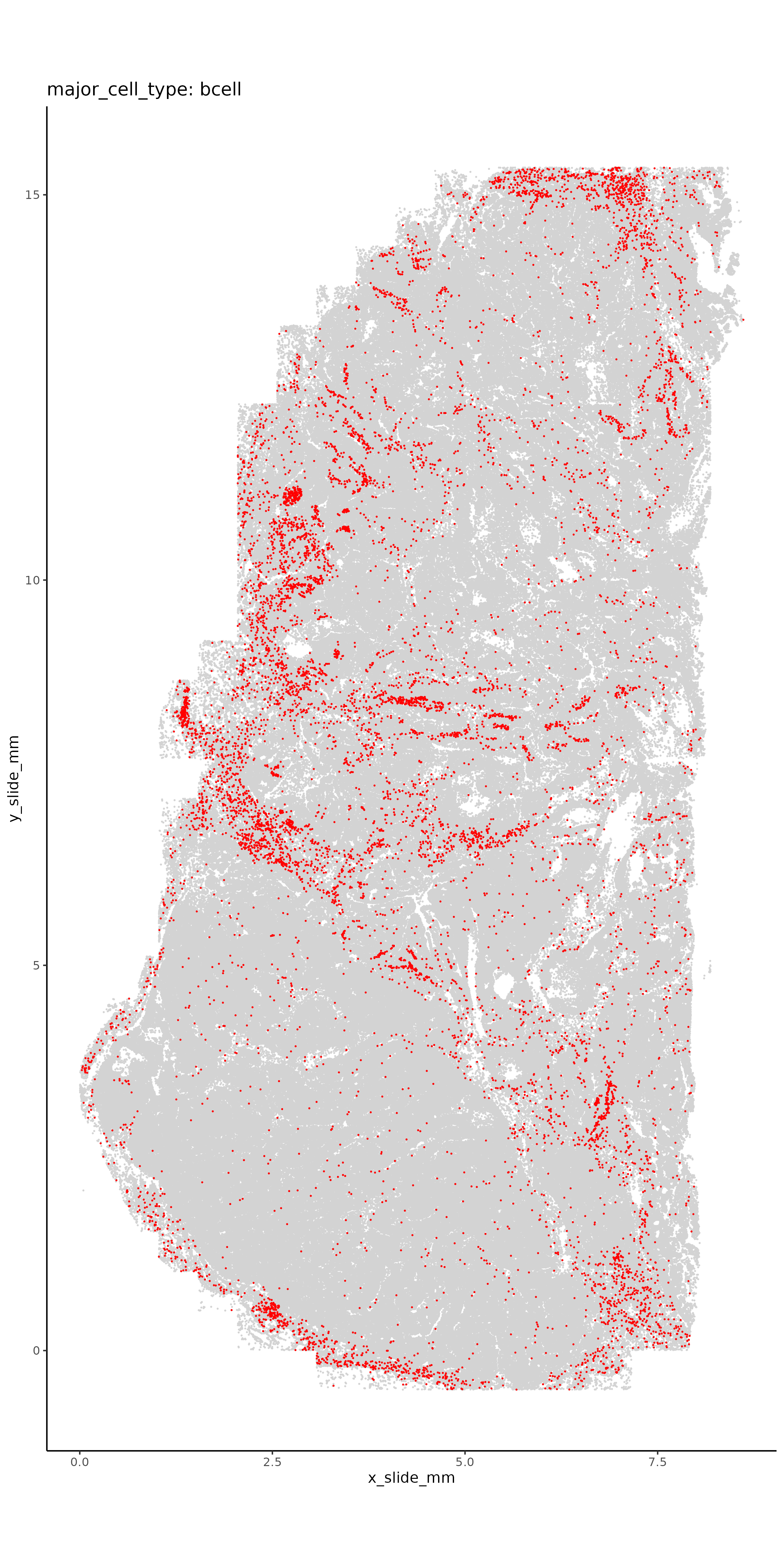
for(ct inc("major_cell_type", "minor_cell_type")){# Plot it in XY space with random colorsset.seed(2025) my_pal <-sample(colors(distinct =TRUE), length(unique(seu.obj@meta.data[,ct])))names(my_pal) <-unique(seu.obj@meta.data[,ct])ggplot(seu.obj@meta.data,aes(x = x_slide_mm, y = y_slide_mm, color =get(ct))) +geom_point(size =0.001) +scale_color_manual(values = my_pal, na.value ="lightgrey", name = ct) +theme_classic() +coord_fixed() +guides(colour =guide_legend(override.aes =list(size=10)))ggsave(filename =paste0(celltyping_dir, "/Plots/XY_", ct, ".png"),width =8, height =16, units ="in")# Plot each cell type separatelyfor (ct1 inunique(seu.obj@meta.data[,ct])){if(is.na(ct1)){next}ggplot(seu.obj@meta.data,aes(x = x_slide_mm, y = y_slide_mm)) +geom_point(size =0.05, color ="lightgrey") +geom_point(data = seu.obj@meta.data %>%filter(get(ct) == ct1),aes(x = x_slide_mm, y = y_slide_mm),size =0.05, color ="red") +theme_classic() +coord_fixed() +ggtitle(paste0(ct, ": ", ct1))ggsave(filename =paste0(celltyping_dir, "/Plots/XY_", ct, "_", ct1, ".png"),width =8, height =16, units ="in") }# Plot it in UMAP spaceDimPlot(seu.obj, group.by = ct, reduction ="umap", label = T) +scale_color_manual(values = my_pal, na.value ="lightgrey") +coord_fixed()ggsave(filename =paste0(celltyping_dir, "/Plots/umap_", ct, ".png"),width =16, height =12, units ="in")# Plot each cell type separately in UMAP space plot.df <- seu.obj@meta.data plot.df$UMAP1 <- seu.obj@reductions$umap@cell.embeddings[,1] plot.df$UMAP2 <- seu.obj@reductions$umap@cell.embeddings[,2]for (ct1 inunique(plot.df[,ct])){ggplot(plot.df,aes(x = UMAP1, y = UMAP2)) +geom_point(size =0.05, alpha =0.5, color ="lightgrey") +geom_point(data = plot.df %>%filter(get(ct) == ct1),aes(x = UMAP1, y = UMAP2),size =0.05, color ="red") +theme_classic() +coord_fixed() +ggtitle(paste0(ct, ": ", ct1))ggsave(filename =paste0(celltyping_dir, "/Plots/UMAP_", ct, "_", ct1, ".png"),width =10, height =8, units ="in") }# Marker heatmap## prepare data for marker gene heatmap: fc_subclus_ctl_gran <-clusterwise_foldchange_metrics(seu.obj[["RNA"]]@counts ,metadata = seu.obj@meta.data ,cluster_column = ct )# subtract background from the mean per-cluster expression profiles: neg_counts = seu.obj@assays$negprobes$countsfor (name inunique(seu.obj@meta.data[,ct])) {if(is.na(name)){next} isthiscelltype <- seu.obj@meta.data[,ct] == name meannegthiscelltype <- Matrix::mean(neg_counts[, isthiscelltype]) fc_subclus_ctl_gran$cluster_expr[fc_subclus_ctl_gran$cluster == name] <-pmax(fc_subclus_ctl_gran$cluster_expr[fc_subclus_ctl_gran$cluster == name] - meannegthiscelltype, 0) }# create the heatmap: hm_lh <-add_ncells(marker_heatmap(fc_subclus_ctl_gran))png(filename =paste0(celltyping_dir, "/Plots/heatmap_", ct, "_negRemoved.png"),width =24, height =8, units ="in", res =300)print(hm_lh)dev.off()# Save results file results_list[paste0(ct, "_color_pal")] <- my_pal}saveRDS(results_list, results_list_file)
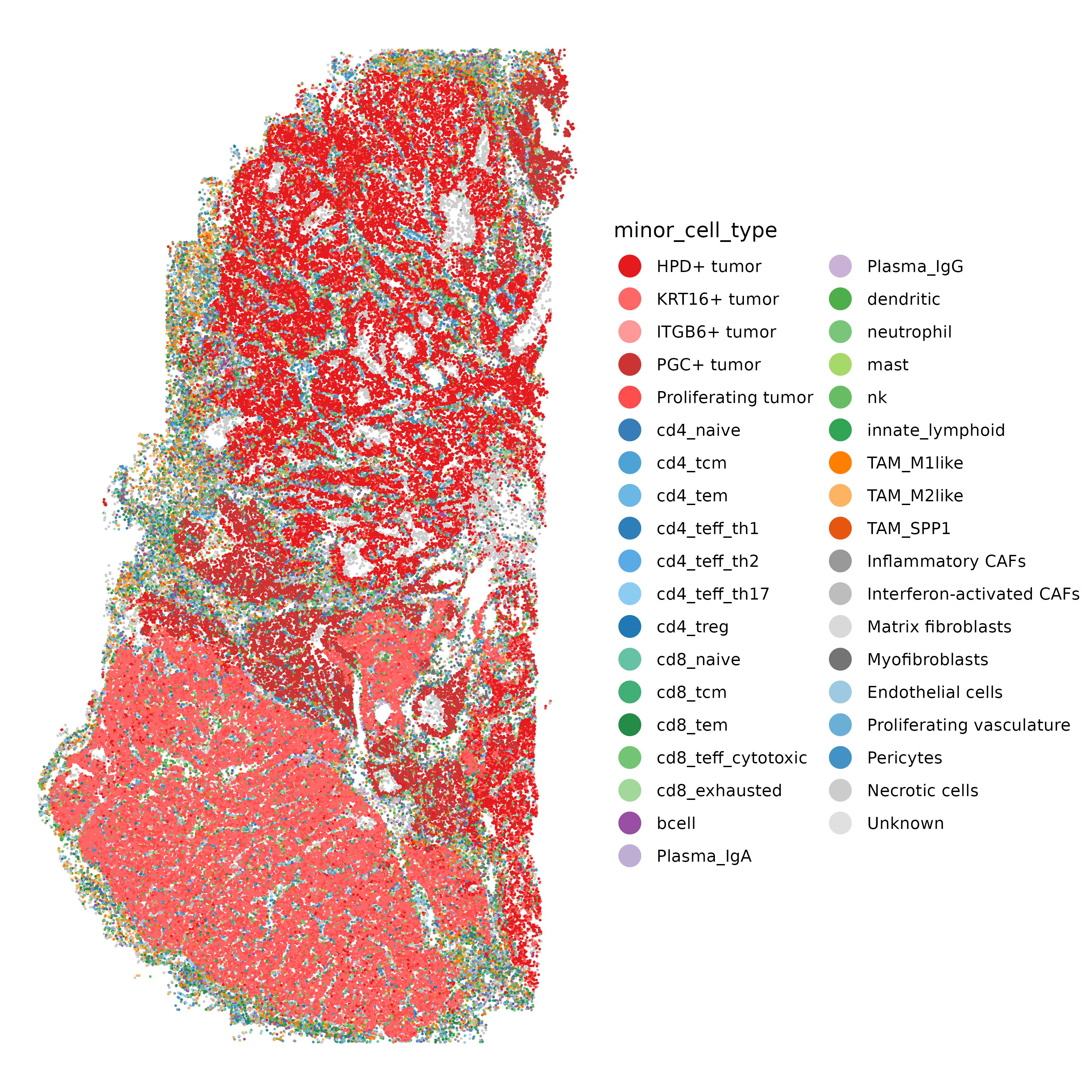
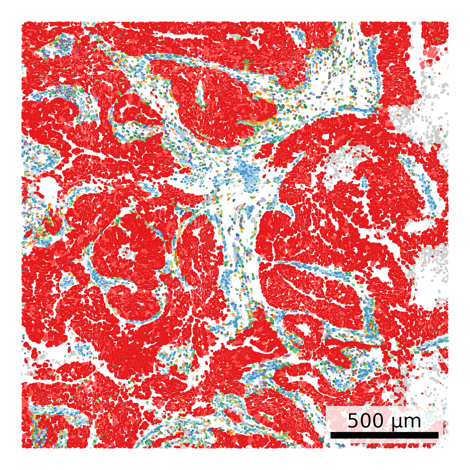
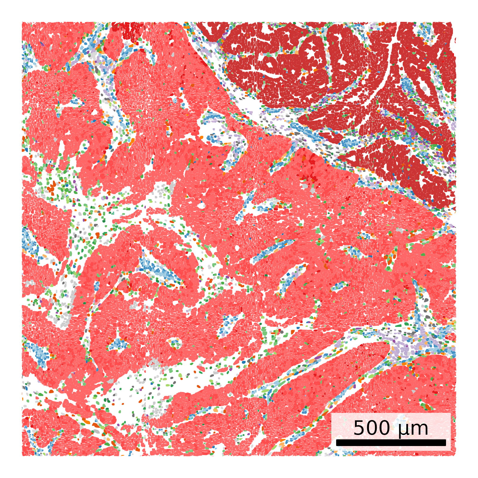
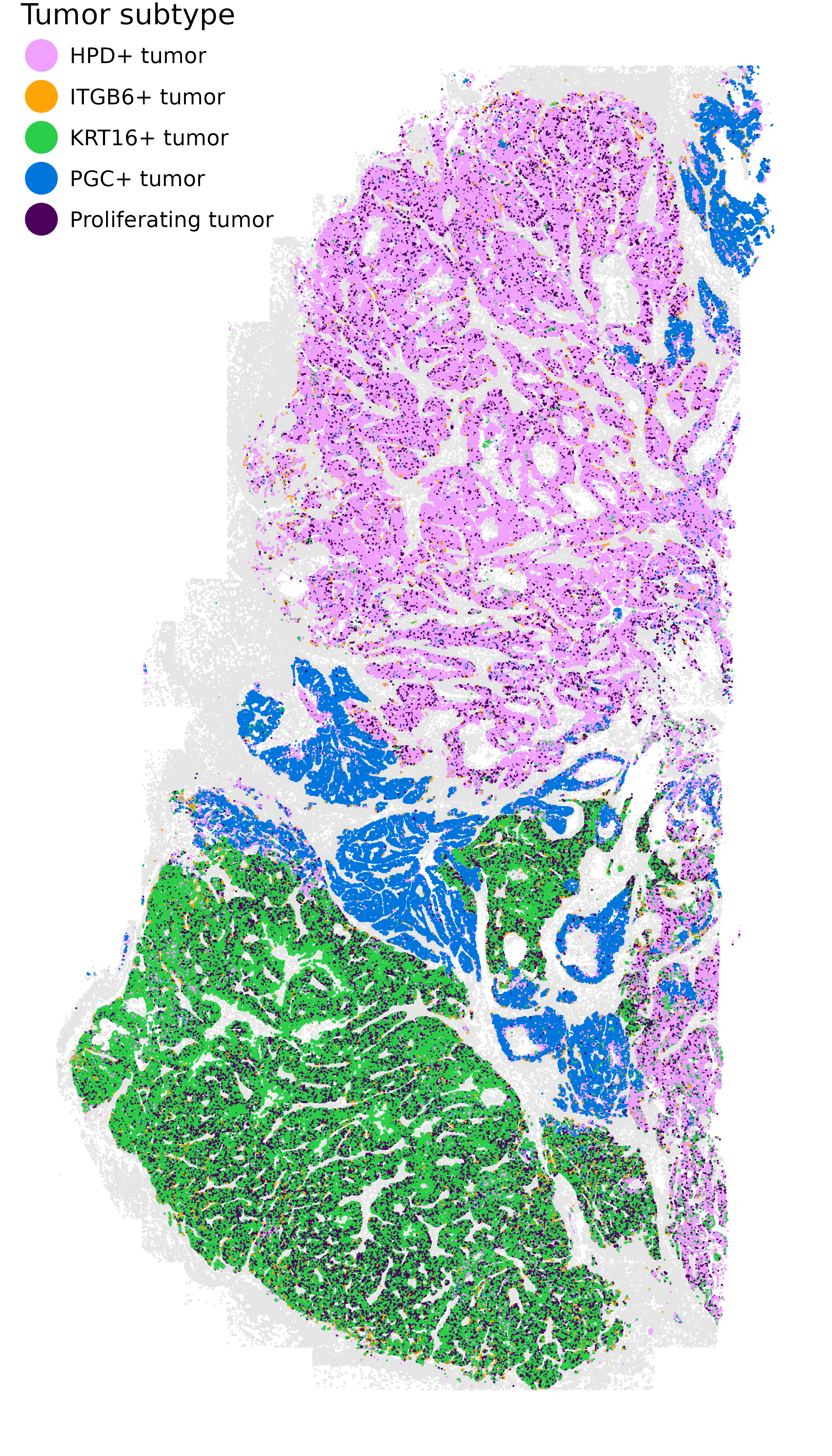
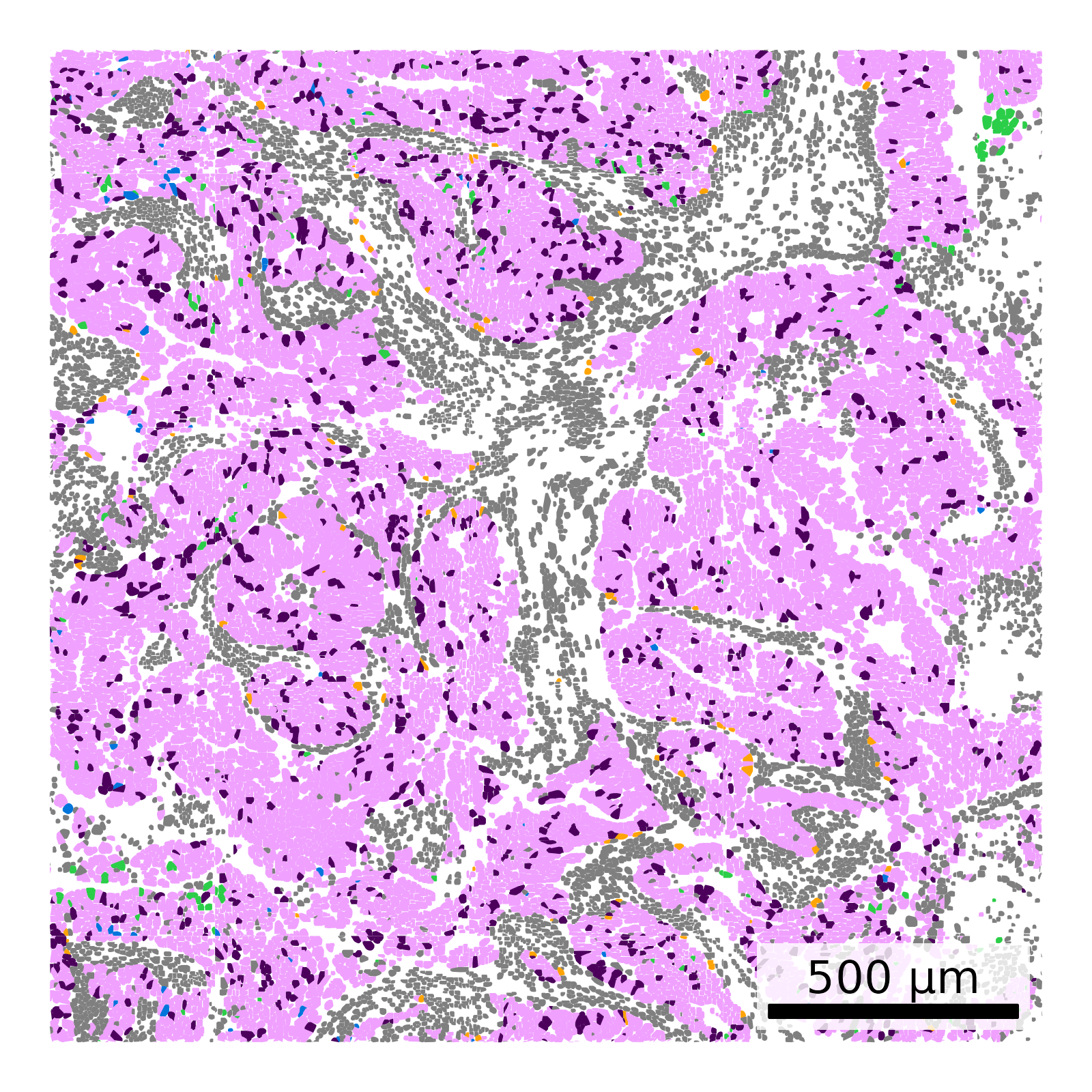
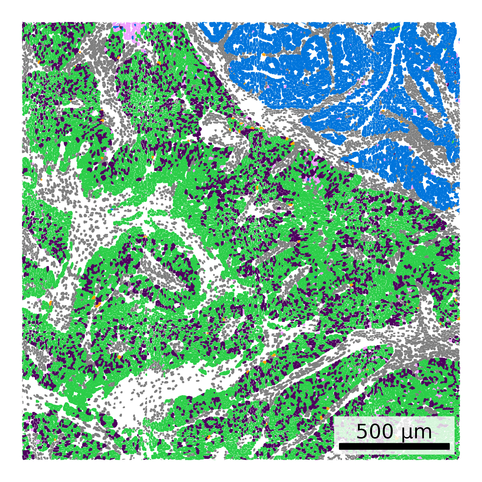
We make a nicer spatial plot of just the five tumor subtypes, using colors chosen to contrast well. There are very few ITGB6+ tumor cells, so in order to ensure that they’re visible we plot them on top.
Show the code
if(!("seu.obj"%in%ls())){ seu.obj <-readRDS(results_list$seurat_file_postCellTyping)}if("LUM+ tumor"%in% seu.obj$minor_cell_type){ seu.obj$minor_cell_type <- dplyr::recode( seu.obj@meta.data$minor_cell_type,"LUM+ tumor"="ITGB6+ tumor" )}# Use alphabet palette, but replace the dark fifth color with a brighter green# Also replace the third brownish color with a brighter redmy_pal <- pals::alphabet(n =5)my_pal[5] <-alphabet(n=7)[7]my_pal[3] <-alphabet(n=25)[15]names(my_pal) <-grep("tumor", unique(seu.obj$minor_cell_type), value = T)# Extract meta datameta <- seu.obj@meta.data# ITGB6+ tumor cells are very rare. Plot on top for visibility.# Plot itggplot(meta %>%filter(major_cell_type !="Tumor"),aes(x = x_slide_mm, y = y_slide_mm)) +geom_point(size =0.01, color ="grey90") +geom_point(data = meta %>%filter(major_cell_type =="Tumor"),aes(x_slide_mm, y_slide_mm, color = minor_cell_type),size =0.01) +geom_point(data = meta %>%filter(minor_cell_type =="ITGB6+ tumor"),aes(x_slide_mm, y_slide_mm, color = minor_cell_type),size =0.01) +scale_color_manual(values = my_pal, name ="Tumor subtype") +theme_void() +coord_fixed() +guides(colour =guide_legend(override.aes =list(size=10))) +theme(legend.position =c(0,1),legend.justification =c(0, 1),legend.text=element_text(size=15),legend.title =element_text(size =20))ggsave(filename =paste0(celltyping_dir, "/Plots/XY_tumor_subclusters_highlighted.png"),width =8, height =14, units ="in")# Plot two zoomed regions with polygonsif(is.null(results_list$zoom_regions)){ zooms =list("zoom1"=list('xmin'=3.25,'xmax'=5.25,'ymin'=9,'ymax'=11,'region'='i'),"zoom2"=list('xmin'=2.5,'xmax'=4.5,'ymin'=3.5,'ymax'=5.5,'region'='ii') ) results_list$zoom_regions <- zoomssaveRDS(results_list, results_list_file)} else{ zooms <- results_list$zoom_regions}# Read in polygonspolygons <-fread(paste0(objects_dir, "/FlatFiles/flatFiles/BreastCancer/BreastCancer-polygons.csv.gz"))polygons$x_slide_mm <- polygons$x_global_px *0.12028/1000polygons$y_slide_mm <- polygons$y_global_px *0.12028/1000# Merge in ctpolygons <-merge(polygons, meta[,c("cell_ID", "minor_cell_type")], by.x ="cell", by.y ="cell_ID", all.y = T)# Plot for each zoom regionfor (zoom in zooms){ idx <-which( polygons$x_slide_mm > zoom$xmin & polygons$x_slide_mm < zoom$xmax & polygons$y_slide_mm > zoom$ymin & polygons$y_slide_mm < zoom$ymax ) scale_bar <-make_scale_bar_r(polygons[idx, c("x_slide_mm")], polygons[idx, "y_slide_mm"])ggplot(polygons[idx,],aes(x_slide_mm, y_slide_mm, group = cell)) +geom_polygon(data = polygons[idx,] %>%filter(!grepl("tumor", polygons[idx, "minor_cell_type"])),aes(x_slide_mm, y_slide_mm, group = cell),fill ="grey90") +geom_polygon(data = polygons[idx,] %>%filter(grepl("tumor", polygons[idx, "minor_cell_type"])),aes(x_slide_mm, y_slide_mm, group = cell, fill = minor_cell_type)) +scale_fill_manual(values = my_pal) +theme_void() +coord_fixed() +theme(legend.position ="none") + scale_bar$bg + scale_bar$rect + scale_bar$labelggsave(paste0(celltyping_dir, "/Plots/XY_tumorsOnly_zoomed_", zoom$region, ".png"),width =4, height =4, units ="in", dpi =400)}
High quality spatial plot of tumor subtypes and two zoomed regions.
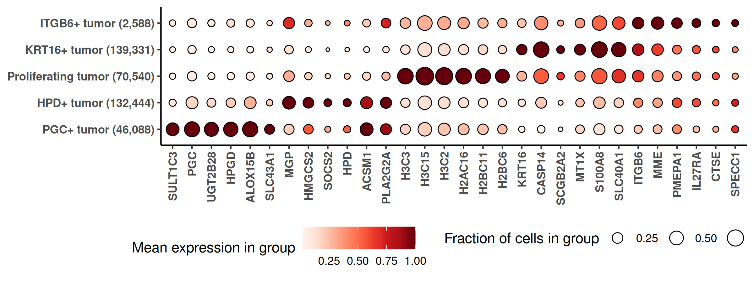
We also make a marker gene heatmap for the tumor subtypes. Use only genes expected to be more highly expressed in tumor cells, as identified with the smiDE overlap metric, than surrounding cells.
Show the code
if(!("seu.obj"%in%ls())){ seu.obj <-readRDS(results_list$seurat_file_postCellTyping)}if("LUM+ tumor"%in% seu.obj$minor_cell_type){ seu.obj$minor_cell_type <- dplyr::recode( seu.obj@meta.data$minor_cell_type,"LUM+ tumor"="ITGB6+ tumor" )}# Identify genes to consider with overlap metricoverlap_metrics <-smiDE::overlap_ratio_metric(assay_matrix = seu.obj@assays$RNA$data,metadata = meta,cluster_col ="major_cell_type",radius =0.05,#split_neighbors_by_colname = "Run_Tissue_name",sdimx_col ="x_slide_mm",sdimy_col ="y_slide_mm" )tumor_genes <- overlap_metrics[major_cell_type=="Tumor"& ratio <=1]$target## prepare data for marker gene heatmap:idx =which(seu.obj$major_cell_type =="Tumor")ct ="minor_cell_type"fc_subclus_ctl_gran <-clusterwise_foldchange_metrics(seu.obj[["RNA"]]@counts[tumor_genes,idx] ,metadata = seu.obj@meta.data[idx,] ,cluster_column = ct)# subtract background from the mean per-cluster expression profiles:negprobes = seu.obj@assays$negprobes$countsfor (name inunique(seu.obj@meta.data[idx,ct])) {if(is.na(name)){next} isthiscelltype <- seu.obj@meta.data[idx,ct] == name meannegthiscelltype <- Matrix::mean(negprobes[,idx][, isthiscelltype]) fc_subclus_ctl_gran$cluster_expr[fc_subclus_ctl_gran$cluster == name] <-pmax(fc_subclus_ctl_gran$cluster_expr[fc_subclus_ctl_gran$cluster == name] - meannegthiscelltype, 0)}# create the heatmap:hm_lh <-marker_heatmap(fc_subclus_ctl_gran, topn =6) +theme(legend.direction ="horizontal", # Arrange items within a legend horizontallylegend.position ="bottom", # Place the entire legend box at the bottomlegend.box ="horizontal"# Arrange multiple legend boxes horizontally )png(filename =paste0(celltyping_dir, "/Plots/heatmap_", ct, "_tumorOnly_negRemoved.png"),width =8, height =3, units ="in", res =300)print(add_ncells(hm_lh))dev.off()