7  Glycolysis

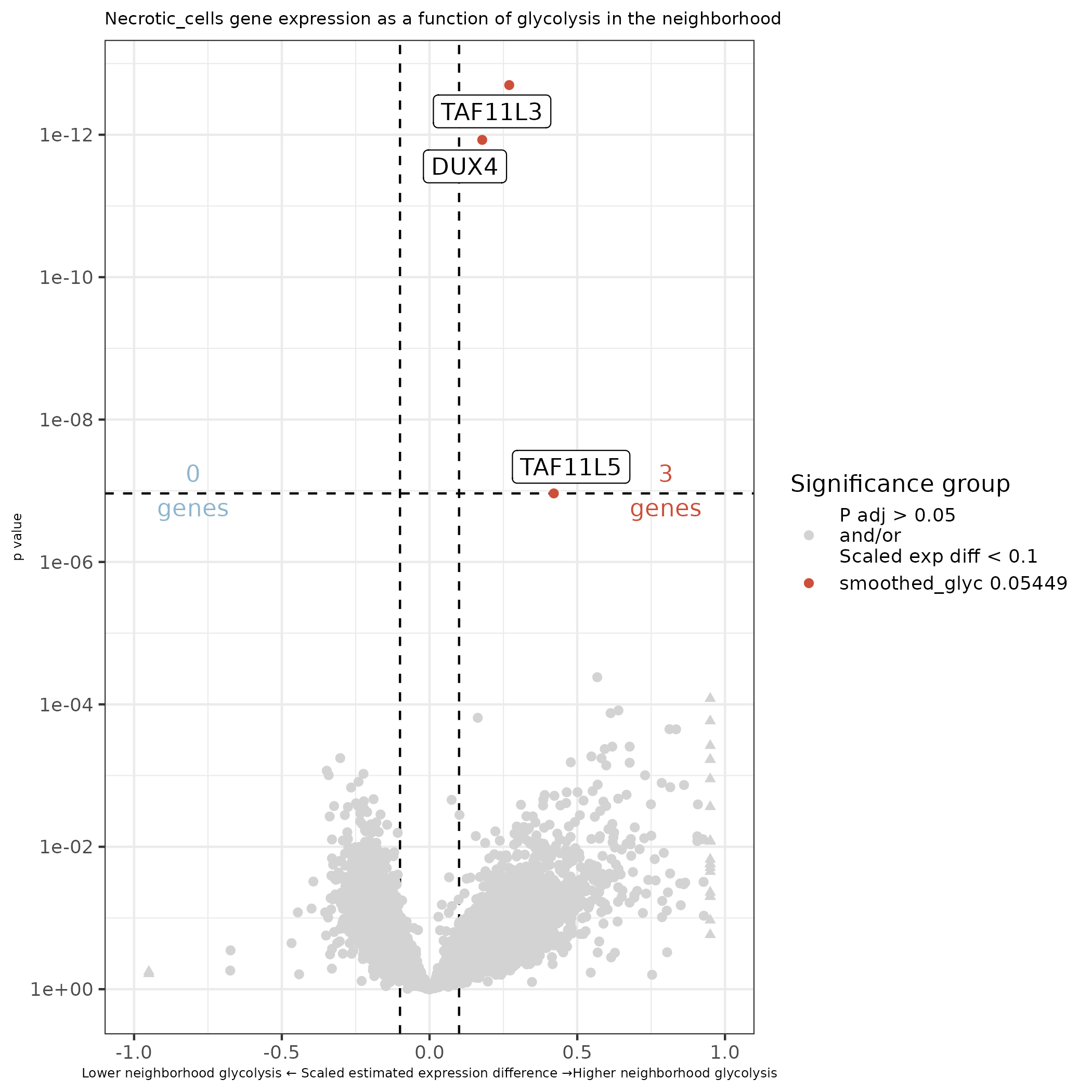
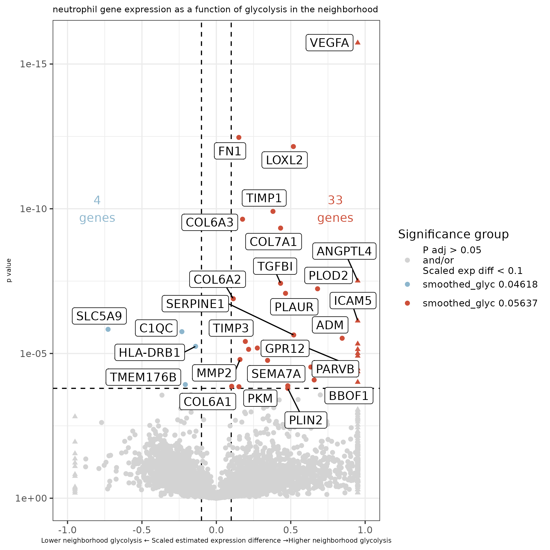
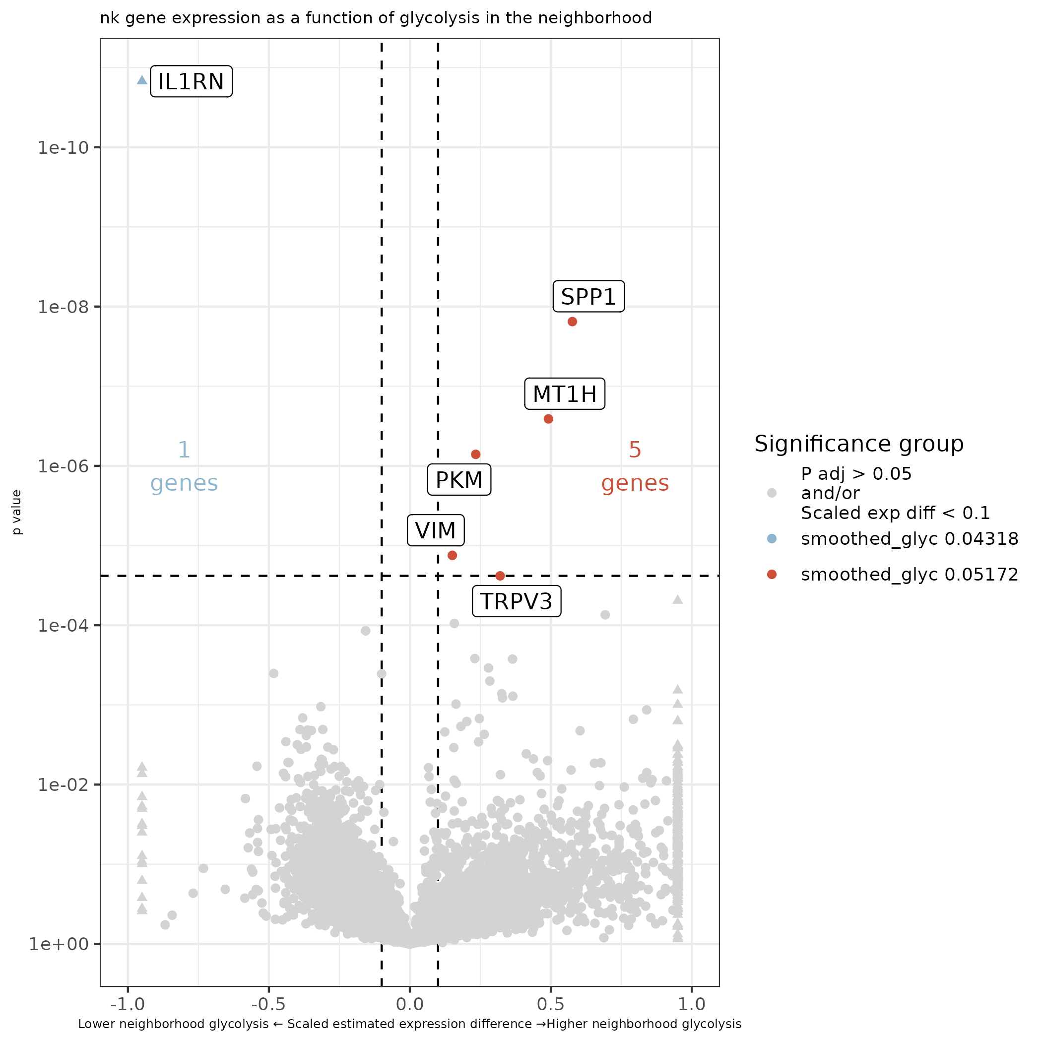
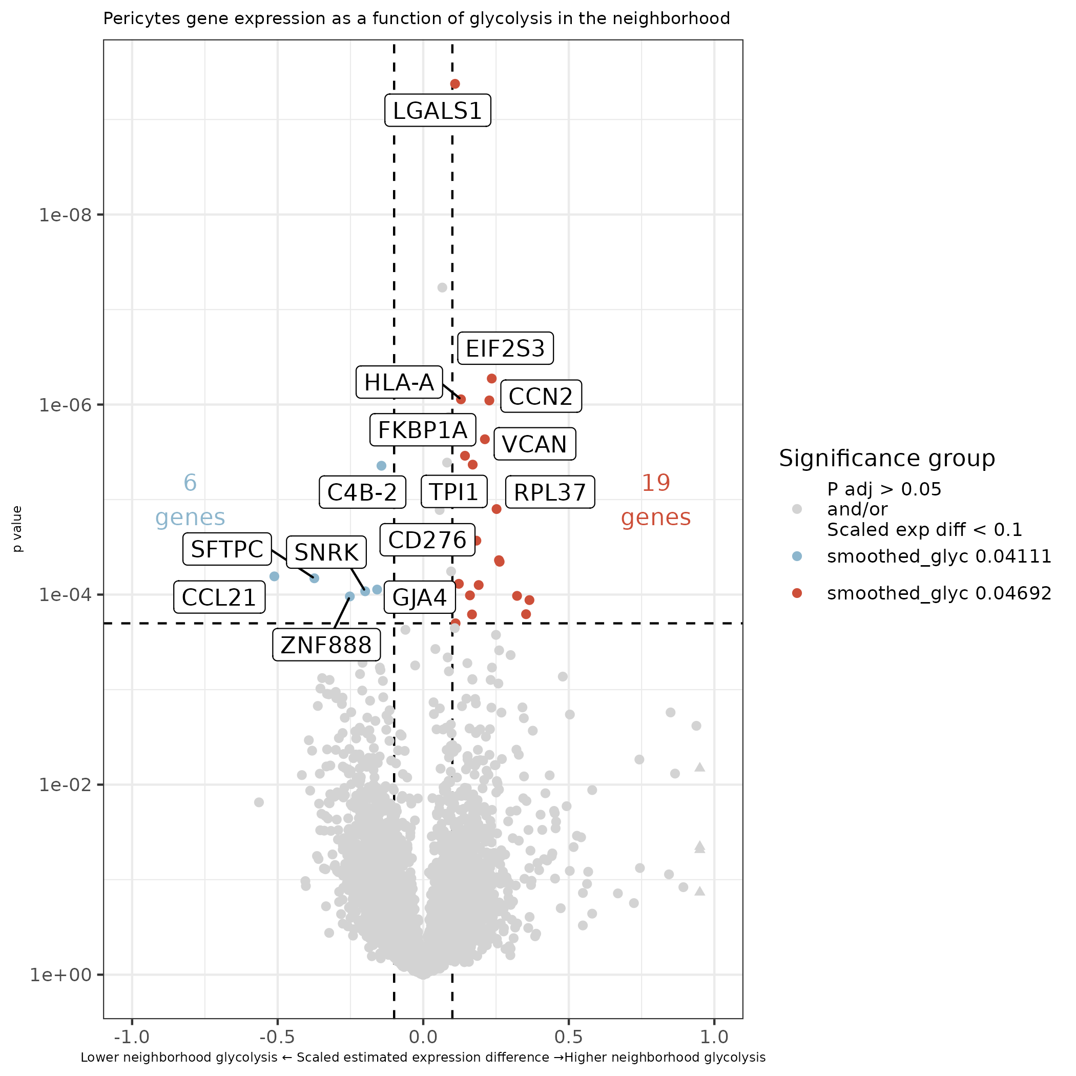
In this section we focus on glycolysis and the impact of the surrounding glycolytic environment on gene expression.

7.1 Smoothed glycolysis pathway scores

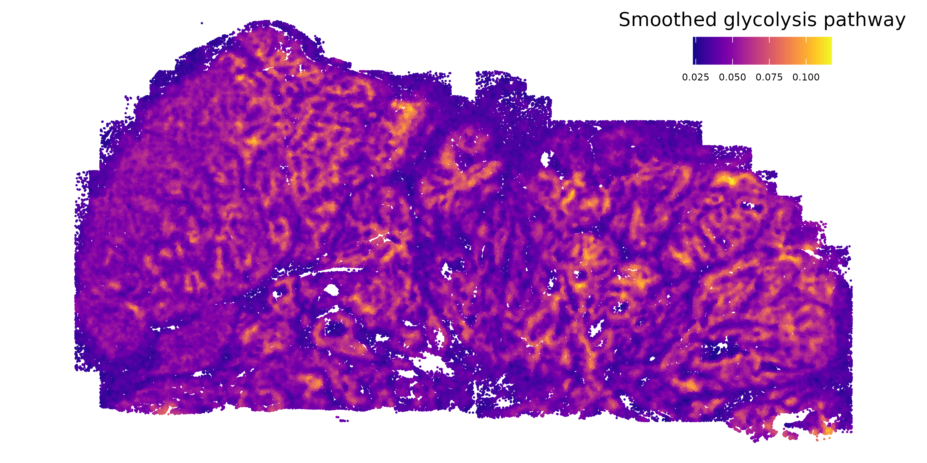
We start by looking at glycolysis in space. We use pathway calculations from AUCell to generate glycolysis pathway scores for every cellular neighborhood.

# if there's no seurat object, read it in
if (!("seu.obj" %in% ls())){
  seu.obj <- readRDS(results_list$seurat_file_postCellTyping)
}

# Read in AUCell results
cells_auc_full <- readRDS(paste0(pathway_dir, "/Data/cellsAUC_full.rds"))

# Extract glycolysis pathway scores
glyc <- cells_auc_full["REACTOME_GLYCOLYSIS",]
meta <- seu.obj@meta.data
meta$glyc <- glyc[meta$cell_ID]

# total expression by cell type:
sumglyc <- by(meta$glyc, meta$major_cell_type, sum)
sumglyc["Tumor"] / sum(sumglyc)

# Calculate smoothed neighborhood expression
xy <- seu.obj@meta.data[,c("x_slide_mm", "y_slide_mm")]
xy$cell_ID <- rownames(xy)

# Use a smoothing function modified from https://nanostring-biostats.github.io/CosMx-Analysis-Scratch-Space/posts/marker-gene-smoothing/
xy_nn <- function(xy, n_neighbors=50){
  xy <- as.data.table(xy)
 
    ## identify nearest n_neighbors (+1 includes the cell as a neighbor to itself)
  nn_xy <- RANN::nn2(xy[,.(x_slide_mm, y_slide_mm)],k = n_neighbors + 1)$nn.idx
  nn_xy <- data.table::melt(cbind(xy[,.(cell_ID)], data.table(nn_xy))
                              , id.vars=c("cell_ID", "V1"))
  colnames(nn_xy) <- c("cell_ID1", "cell_ID1_idx", "neighbor", "cell_ID2_idx")
  nn_xy <- merge(nn_xy
                   , nn_xy[,.(cell_ID2=cell_ID1, cell_ID2_idx=cell_ID1_idx)][
                     ,unique(.SD)],by="cell_ID2_idx")
  
  ## Cell x cell neighbor indicator matrix
  wxy <- Matrix::sparseMatrix(i = c(unique(nn_xy$cell_ID1_idx), nn_xy$cell_ID2_idx)
                                ,j=c(unique(nn_xy$cell_ID1_idx), nn_xy$cell_ID1_idx)
                                ,x=1)
  
  rownames(wxy) <- colnames(wxy) <- nn_xy[order(nn_xy$cell_ID1_idx),unique(cell_ID1)]
  
  ## Column standardize, so that columns (cells) sum to 1, and each neighbor given equal weight.
  mxy <- Matrix::sparseMatrix(i=1:ncol(wxy)
                                ,j=1:ncol(wxy)
                                ,x=1/Matrix::colSums(wxy)
                                )
  dimnames(mxy) <- dimnames(wxy)
  smoother <- mxy %*% wxy
  smoother <- smoother[,xy$cell_ID]
  return(smoother)
}

# Smoothed glycolysis pathway
smoother <- xy_nn(xy)
smoothed_glyc <- meta[,"glyc"] %*% smoother

# Save this smoothed glycolysis pathway score
saveRDS(smoothed_glyc, file = paste0(metabolism_dir, "/Data/xy_smoothed_glycolysis.rds"))

# Plot smoothed glycolysis in space
meta$smoothed_glyc <- smoothed_glyc[1,]
ggplot(meta, aes(x = y_slide_mm, y = -x_slide_mm, # Plotting on its side
                 color = smoothed_glyc)) +
  geom_point(size = 0.01) +
  scale_color_viridis(option = "plasma", name = "Smoothed glycolysis pathway") +
  coord_fixed() +
  theme_void() +
  theme(legend.position = c(0.85, 0.9), 
        legend.direction = "horizontal", 
        legend.title.position = "top",
        legend.text = element_text(size = 6),
        legend.title = element_text(hjust = 0.5, size = 12))
  
ggsave(filename = paste0(metabolism_dir, "/Plots/XY_smoothed_glycolysis.png"),
       width = 8, height = 4, units = "in", dpi = 400)

Here is the smoothed glycolysis pathway in space. Enrichment is prominent throughout the tumor.

knitr::include_graphics(paste0(metabolism_dir, "/Plots/XY_smoothed_glycolysis.png"))

7.2 Differential expression as a function of neighborhood glycolysis

Here we run DE on every cell type to try to understand how every cell type changes as a function of glycolysis levels in the neighborhood it finds itself in. The prediction is that we might find some genes that are consistently up or down regulated across all or many cell types. This might also point us towards cell types that are more or less responsive / susceptible to the surrounding glycolysis environment. As additional factors in our model, we also include niche and the number of each tumor cell type in the 50 nearest neighbors. For speed in making this many comparisons, we work with normalized counts and a gaussian model.

if (!("seu.obj" %in% ls())){
  seu.obj <- readRDS(results_list$seurat_file_postCellTyping)
}

## Isolate meta data and add neighborhood glycolysis activity
meta <- seu.obj@meta.data

smoothed_glyc <- readRDS(file = paste0(metabolism_dir, "/Data/xy_smoothed_glycolysis.rds"))

meta$smoothed_glyc <- smoothed_glyc[1,meta$cell_id]

# Add number of each type of tumor cell in 50 nearest neighbors
coords <- as.matrix(meta[, c("x_slide_mm", "y_slide_mm")])
K <- 50
idx <- FNN::get.knn(coords, k = K)$nn.index  # (N x K), self is not included here

# Count cells in neighborhood
types   <- as.character(meta$minor_cell_type)
targets <- c("LUM+ tumor","HPD+ tumor","PGC+ tumor","KRT16+ tumor","Proliferating tumor")

neighbor_counts <- lapply(targets, function(lbl) {
  is_target <- (types == lbl)
  mat <- matrix(is_target[idx], nrow = nrow(idx), ncol = ncol(idx))
  rowSums(mat)
})
names(neighbor_counts) <- targets

meta$neighboring_lum  <- neighbor_counts[["LUM+ tumor"]]
meta$neighboring_hpd  <- neighbor_counts[["HPD+ tumor"]]
meta$neighboring_pgc  <- neighbor_counts[["PGC+ tumor"]]
meta$neighboring_krt  <- neighbor_counts[["KRT16+ tumor"]]
meta$neighboring_prol <- neighbor_counts[["Proliferating tumor"]]

# Add novae domain
novae_9 <- readRDS(paste0(niche_dir, "/Data/novae_domains_9_assignments.rds"))
meta$novae <- novae_9[rownames(meta)]

## Prep pre-de files that are conserved across cell types

# Pre-de find neighbors
pre_de_obj <- pre_de(
  metadata = meta,
  cell_type_metadata_colname = "minor_cell_type",
  mm_radius = 0.05,
  sdimx_colname = "x_slide_mm",
  sdimy_colname = "y_slide_mm",
  verbose = TRUE
)

# Save pre-de results
saveRDS(pre_de_obj, file = paste0(metabolism_dir, "/Data/pre_de_obj.rds"))

# Run overlap filter

overlap_metrics <- 
overlap_ratio_metric(assay_matrix = seu.obj@assays$RNA$data,
                           metadata = meta,
                           cluster_col = "minor_cell_type",
                           radius = 0.05,
                           sdimx_col = "x_slide_mm",
                           sdimy_col = "y_slide_mm"
                           )

# Save overlap metrics
saveRDS(overlap_metrics, file = paste0(metabolism_dir, "/Data/overlap_metrics.rds"))

# Add total counts to metadata as DE expects
meta$totalcounts = meta$nCount_RNA

# Work with total count normalized data
counts <- seu.obj@assays$RNA$counts
scaling_factor <- mean(seu.obj@meta.data$nCount_RNA)
norm <- counts %*% 
  Matrix::Diagonal(x = scaling_factor/seu.obj@meta.data$nCount_RNA,
                         names=colnames(counts)) 
 

# Iterate through each cell type

for(ct in unique(meta$minor_cell_type)){
  print(paste0("Starting cell type ", ct, " at ", Sys.time()))
  
  # Only analyze genes with overlap ratio less than or equal to 1
  analysis_genes <- overlap_metrics[minor_cell_type == ct & ratio <= 1]$target
  
  # Extract counts for analysis genes only
  sub_counts <- norm[analysis_genes,]
  
  # DE test dependence on neighborhood glycolysis
  de_obj <- smiDE::smi_de(
    assay_matrix = sub_counts,
    metadata = meta[which(meta[,"minor_cell_type"]== ct),],
    formula = ~RankNorm(otherct_expr) + smoothed_glyc + novae + neighboring_lum + neighboring_hpd + neighboring_pgc + neighboring_krt + neighboring_prol,
    pre_de_obj = pre_de_obj,
    groupVar = "smoothed_glyc",
    neighbor_expr_cell_type_metadata_colname = "minor_cell_type",
    neighbor_expr_totalcount_normalize = FALSE,
    neighbor_expr_totalcount_scalefactor = NULL,
    family = "gaussian",
    targets = analysis_genes,
    nCores = 24
  )
  
  # Save objects
  saveRDS(de_obj, file = paste0(metabolism_dir, "/Data/ct_", gsub("\\+", "", gsub(" ", "_", ct)), "_smoothedGlycolysis_de_obj_plusNicheNeighborTumor.rds"))
}

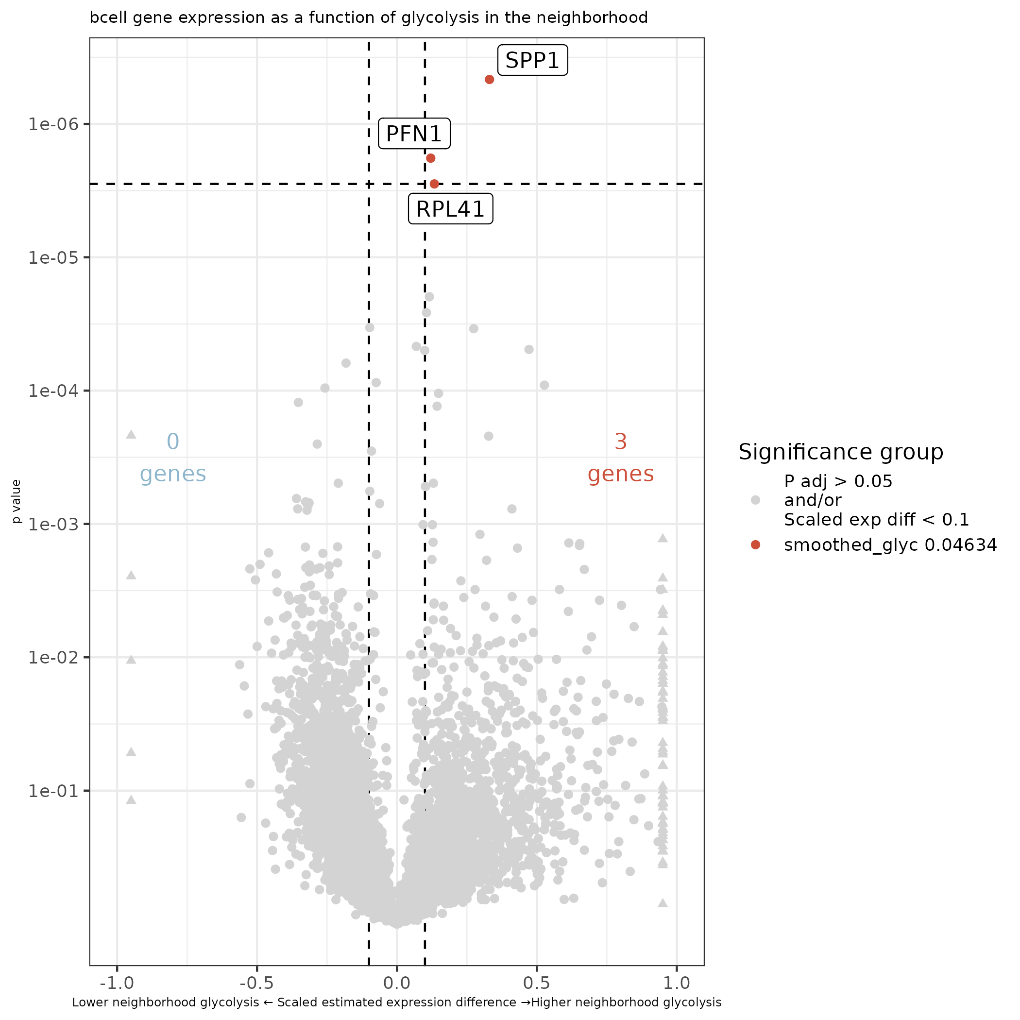
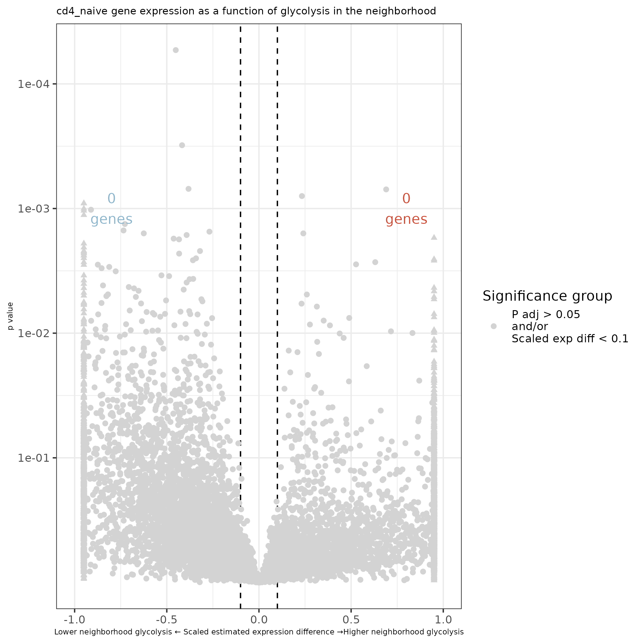
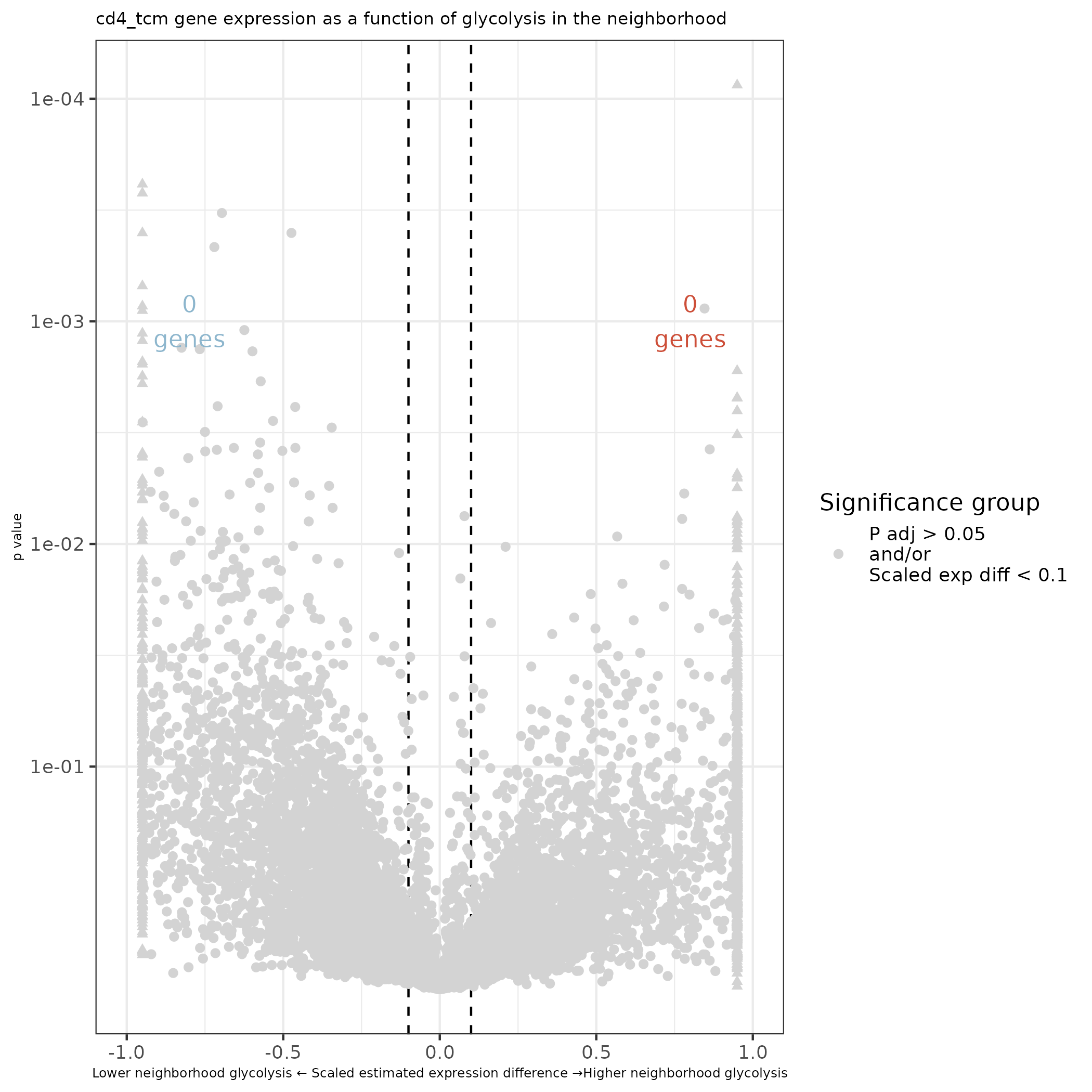
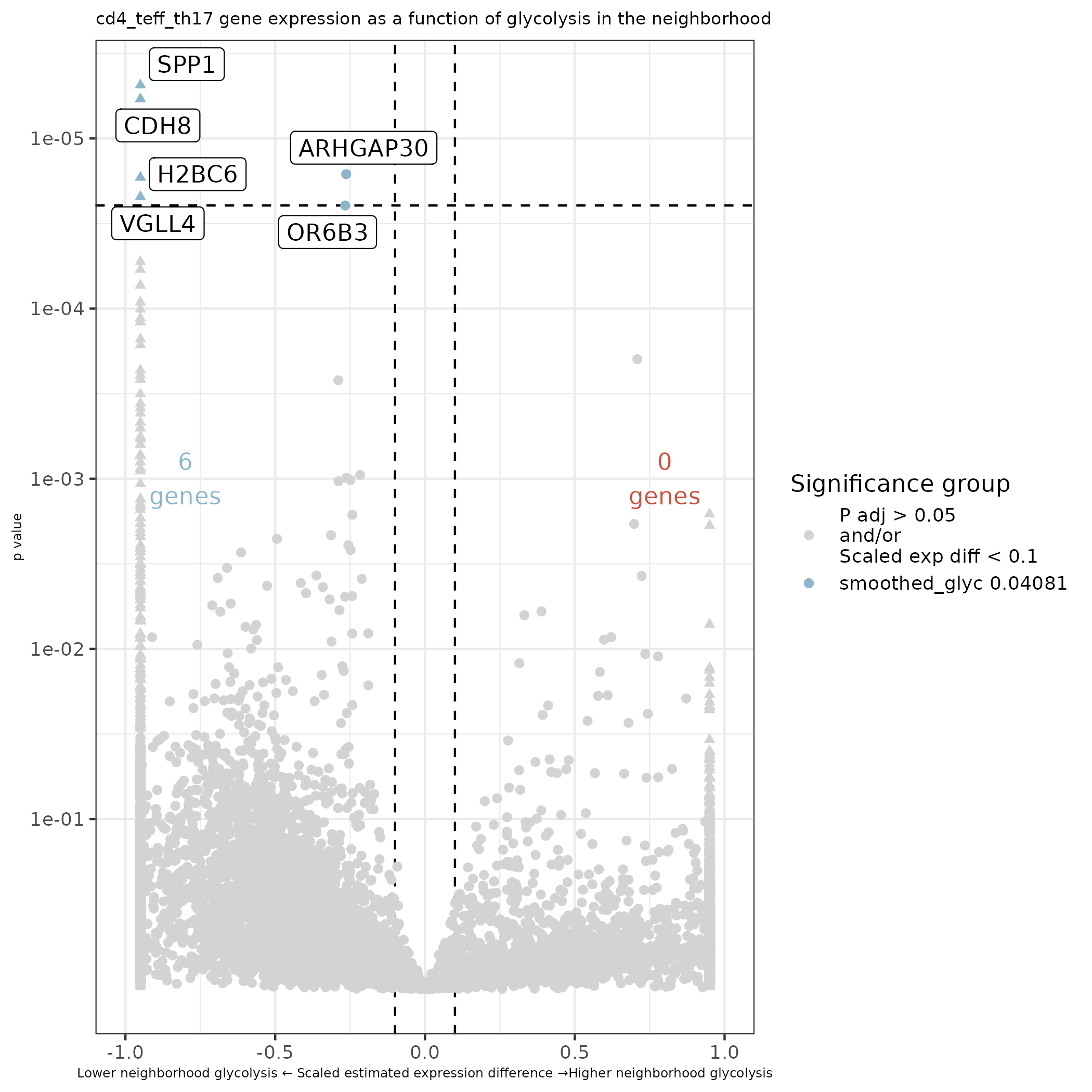
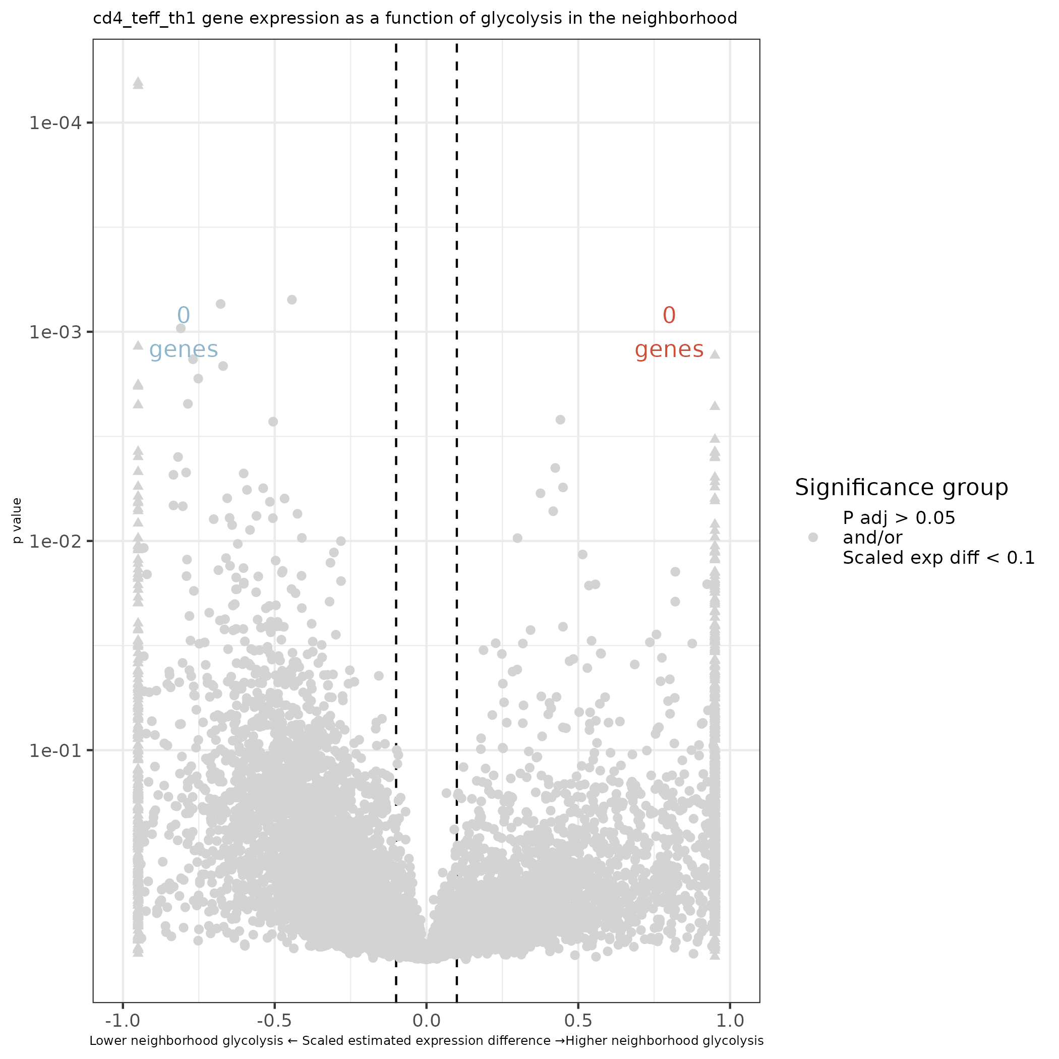
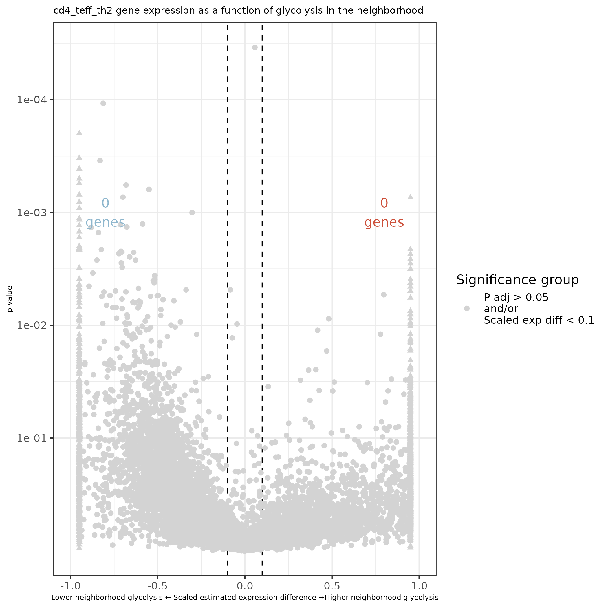
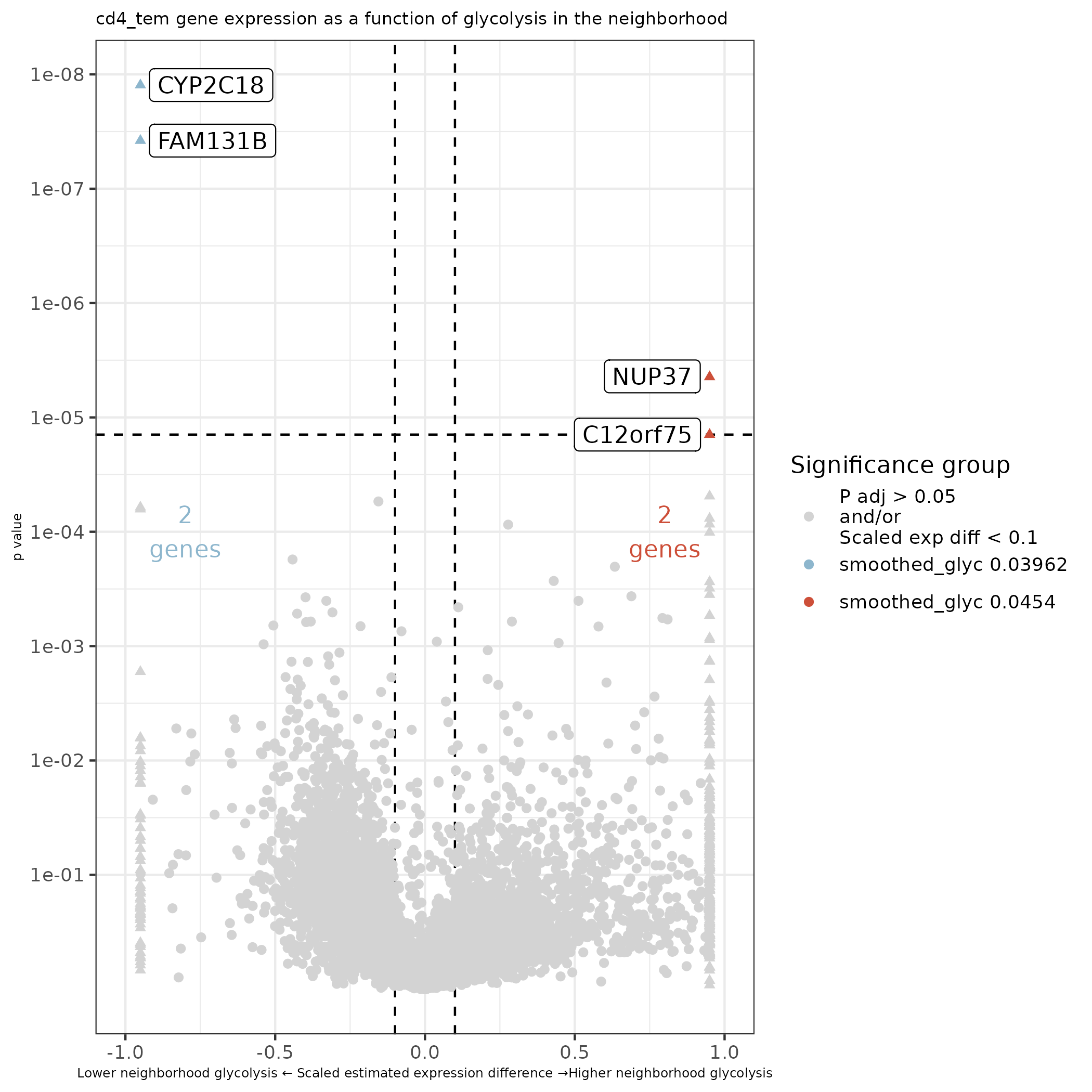
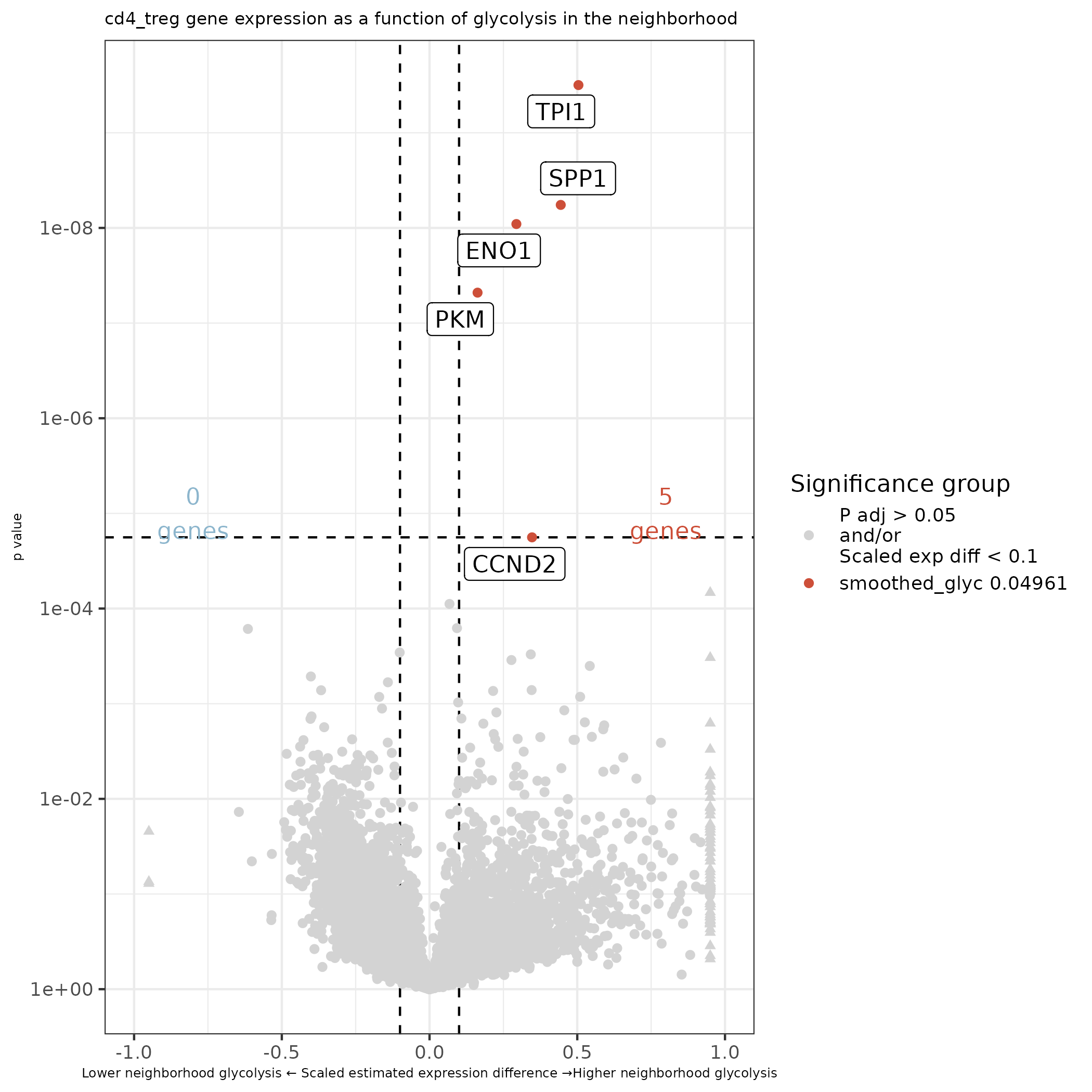
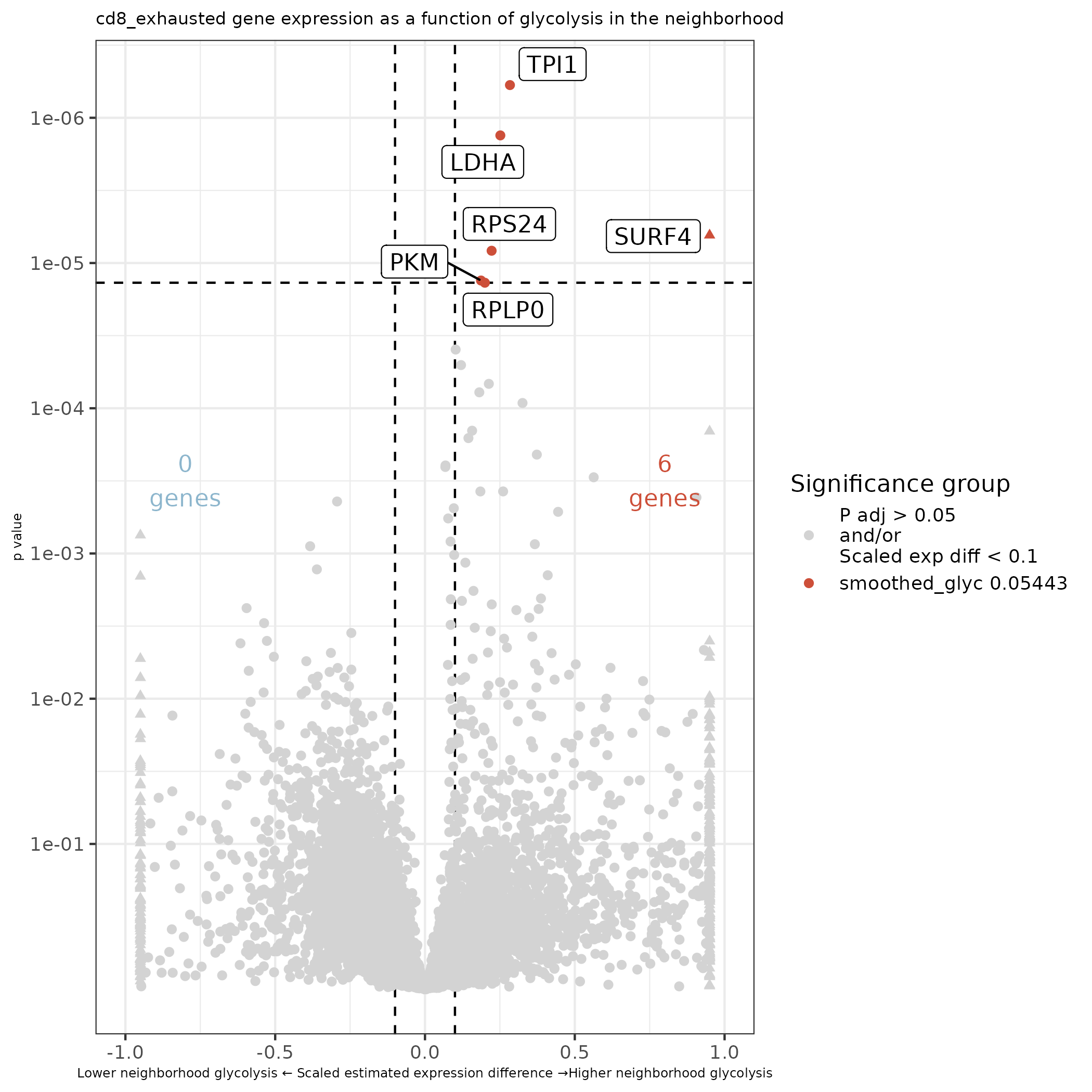
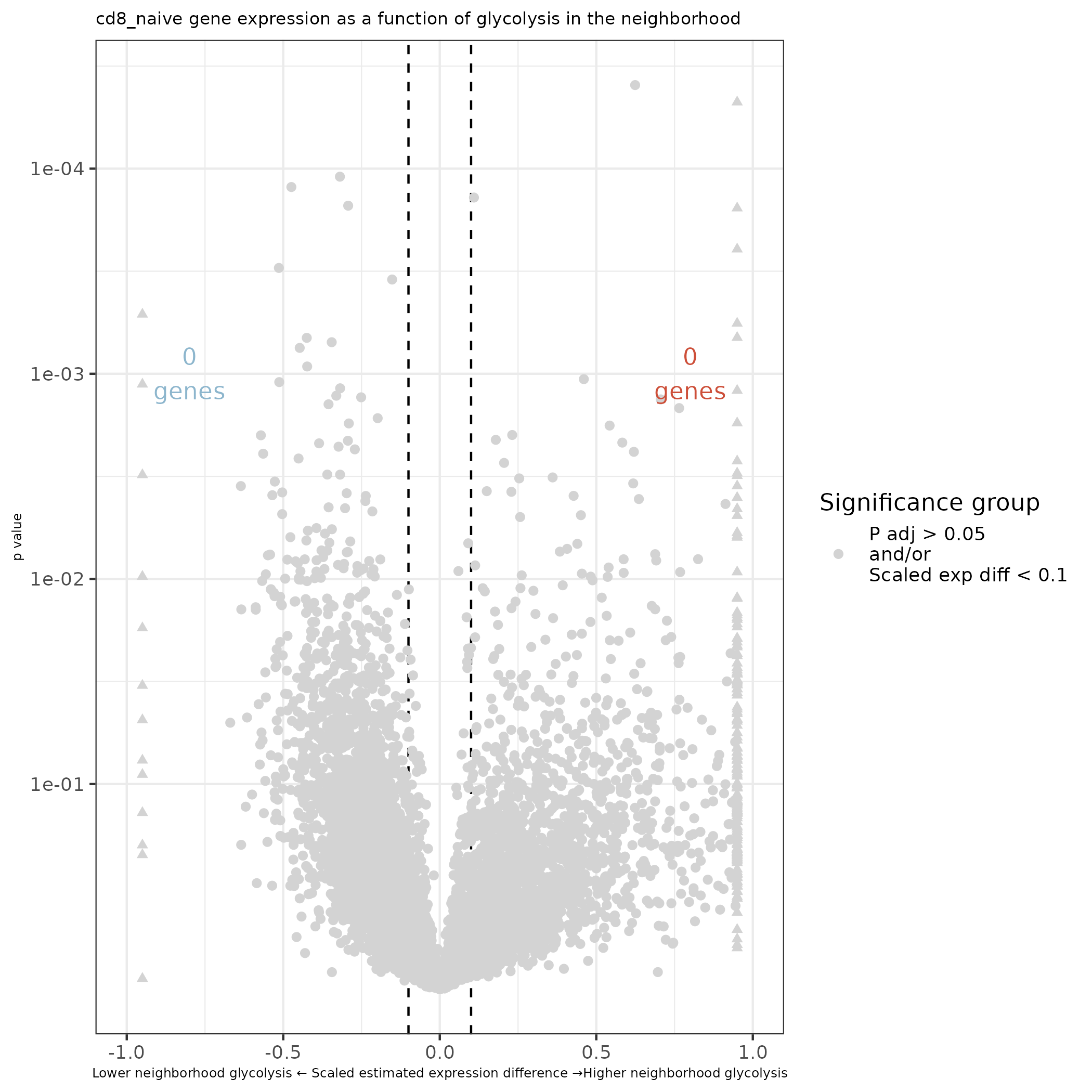
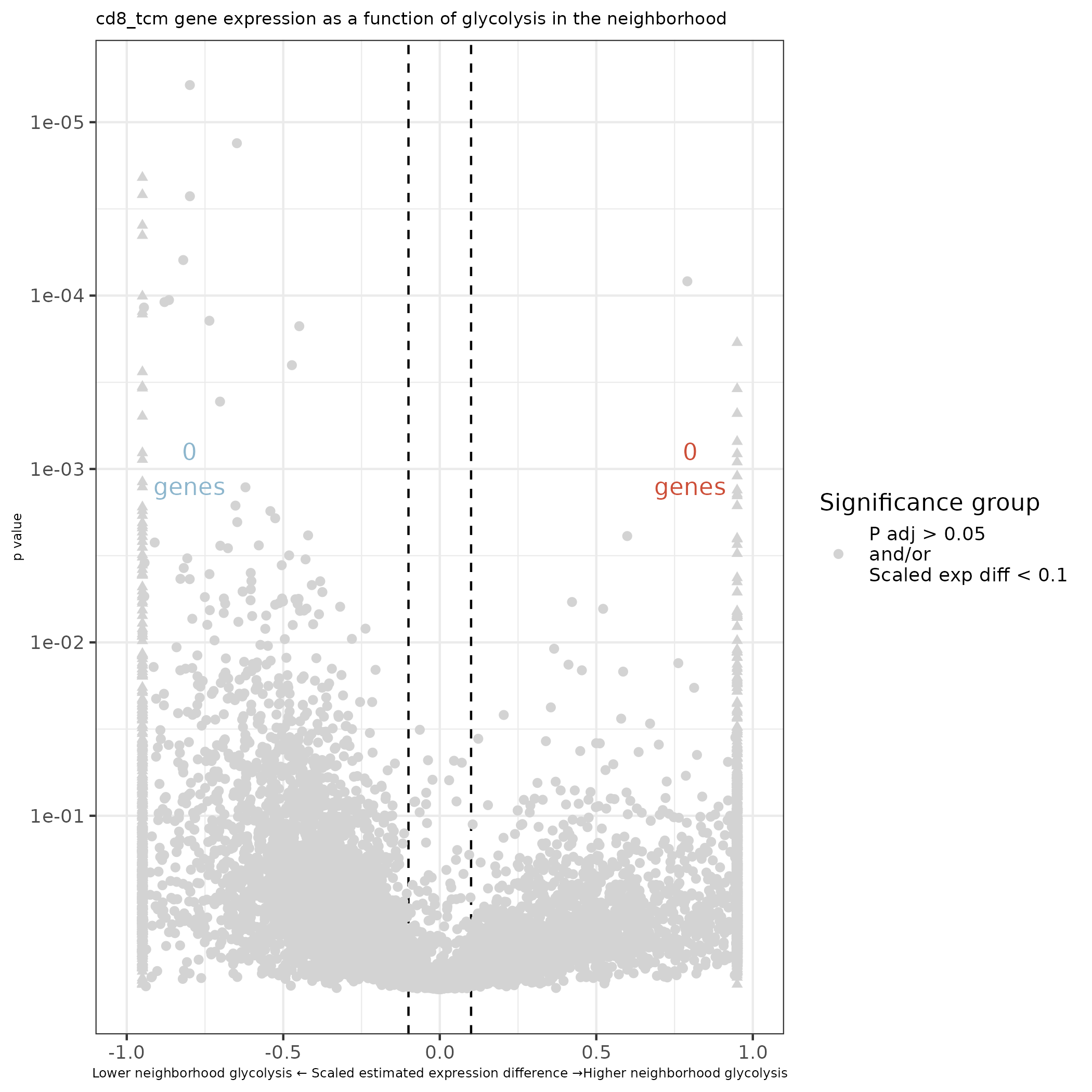
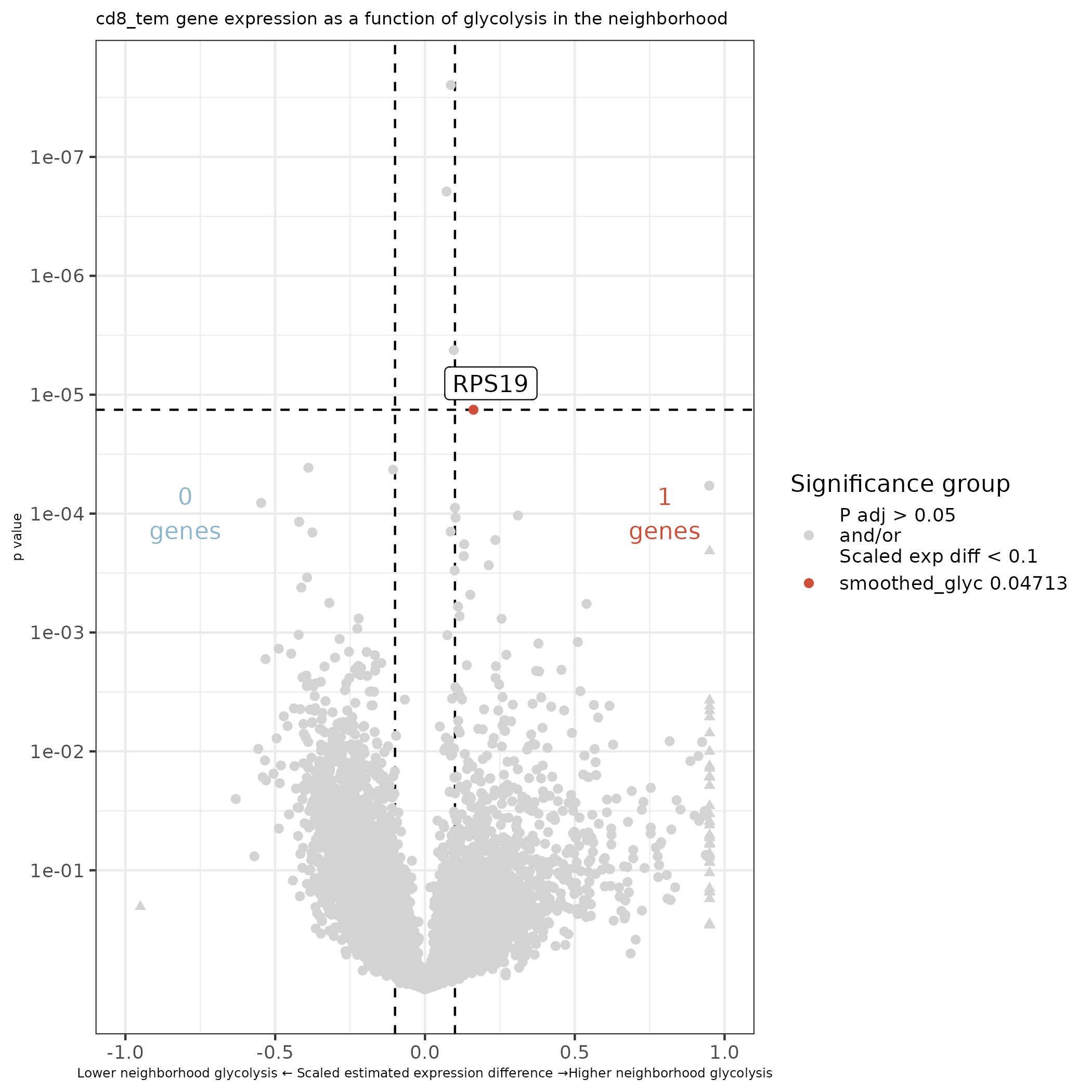
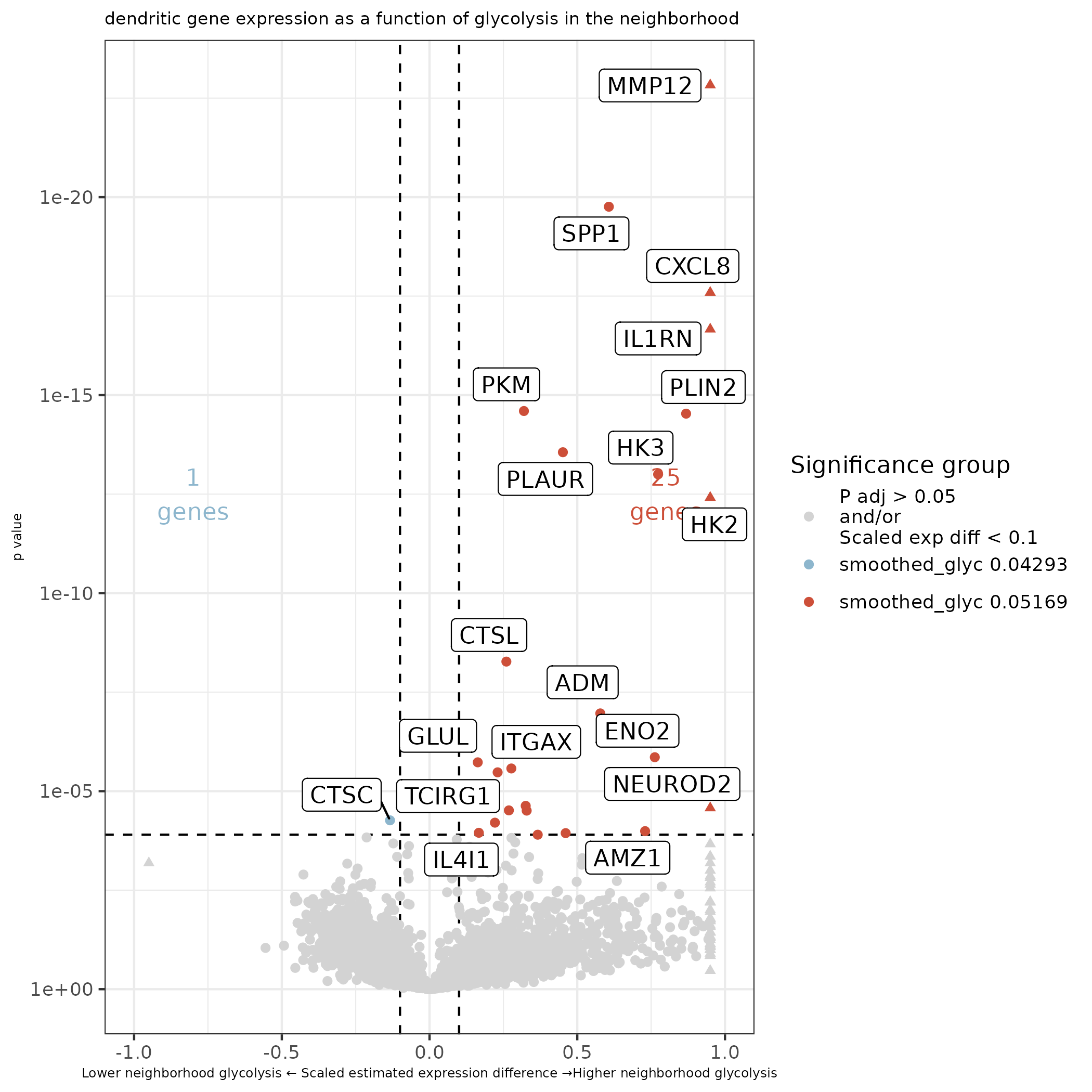
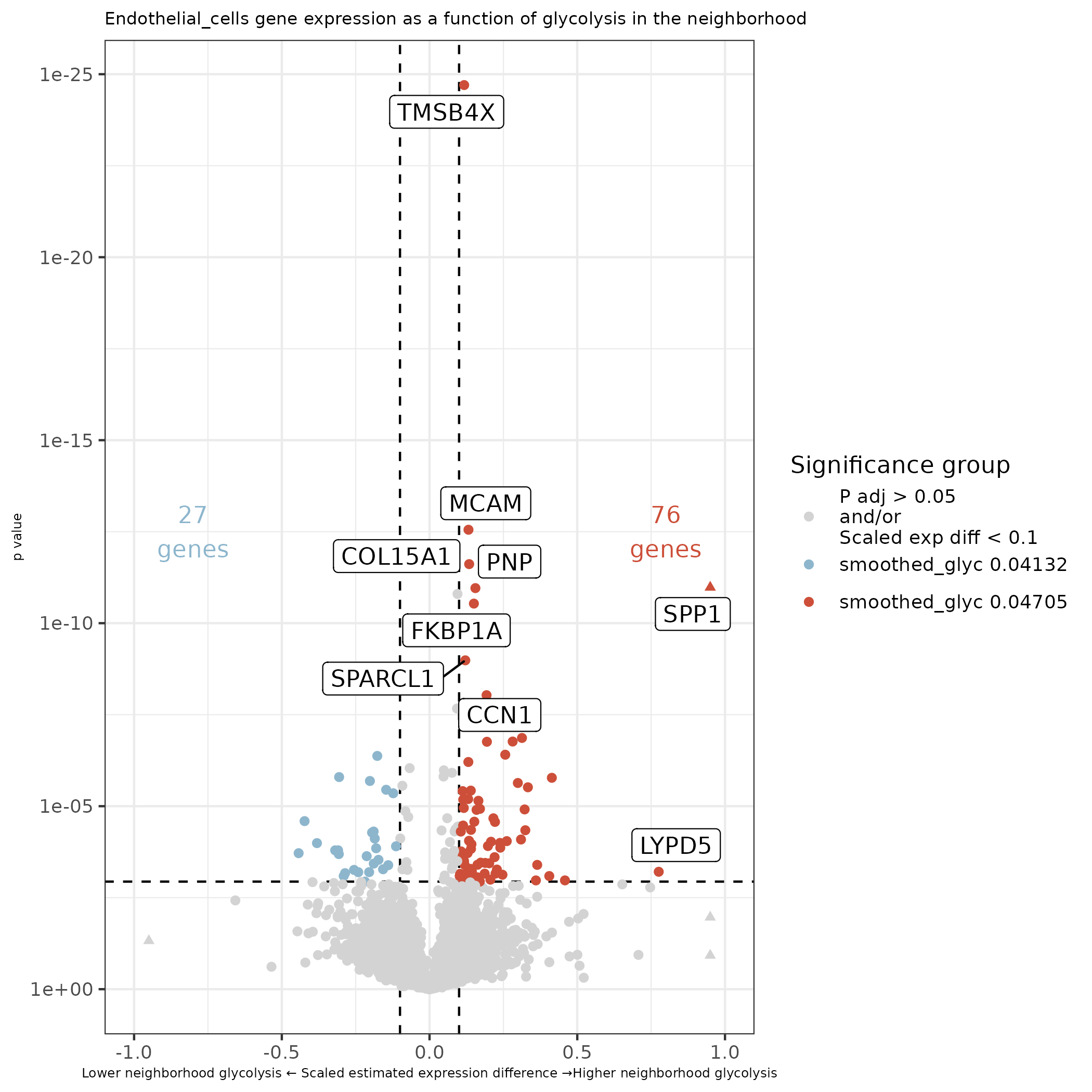
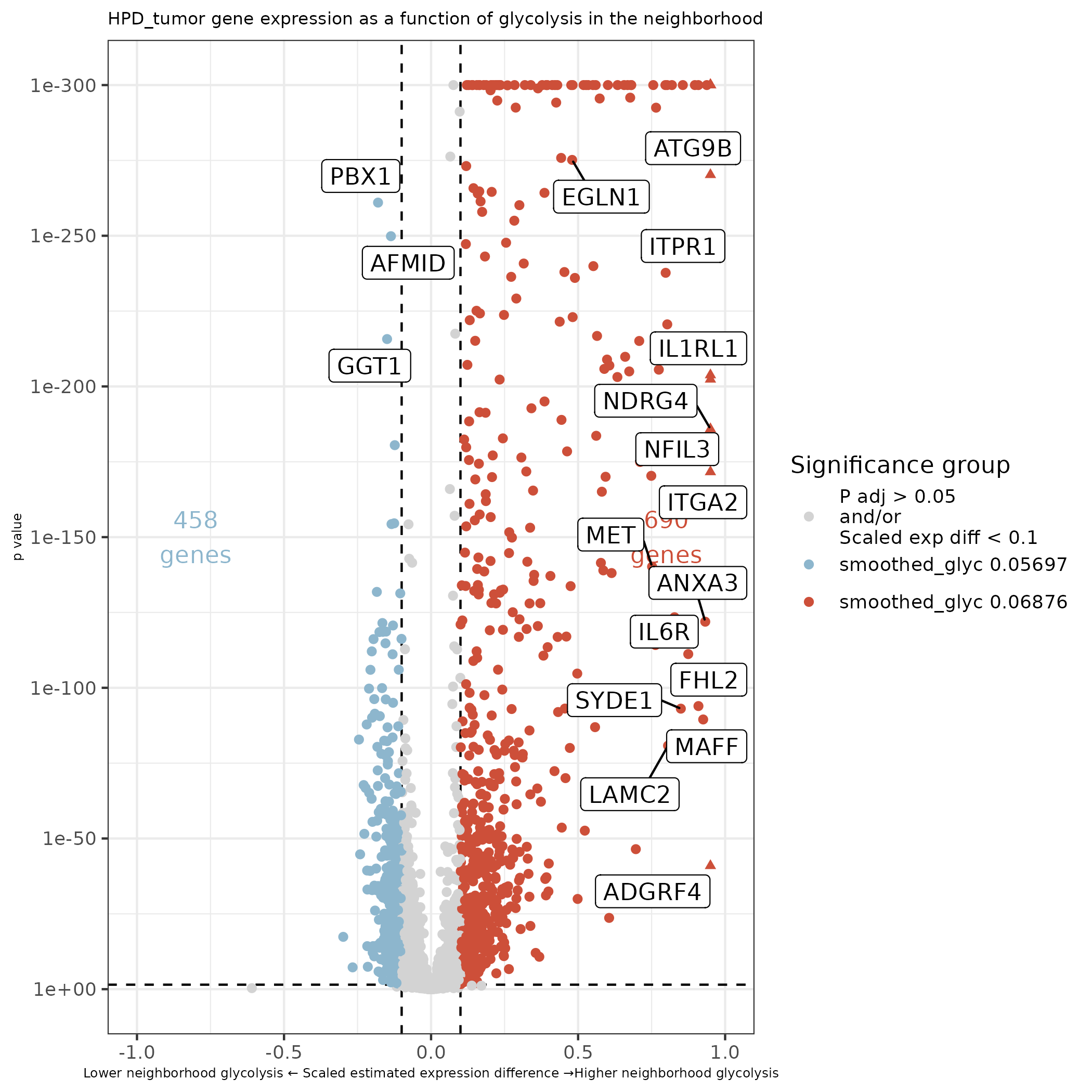
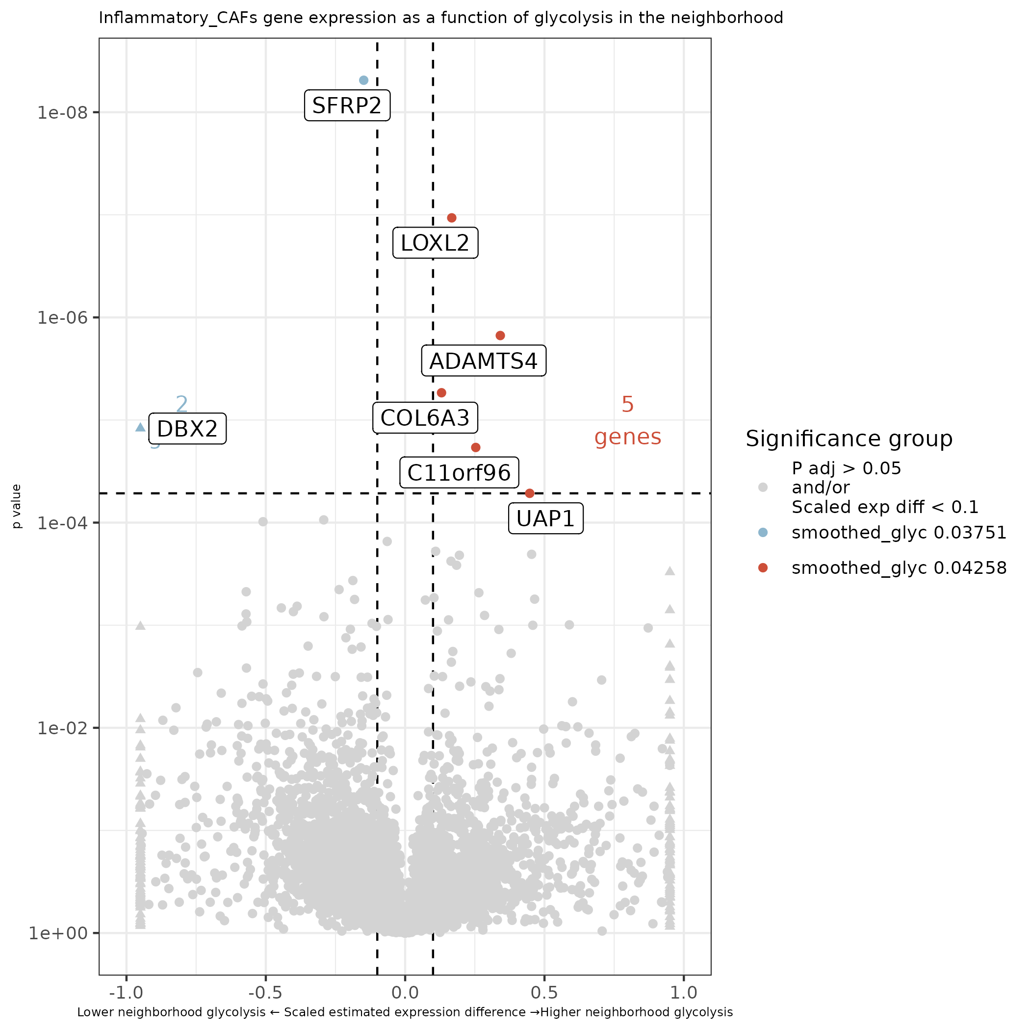
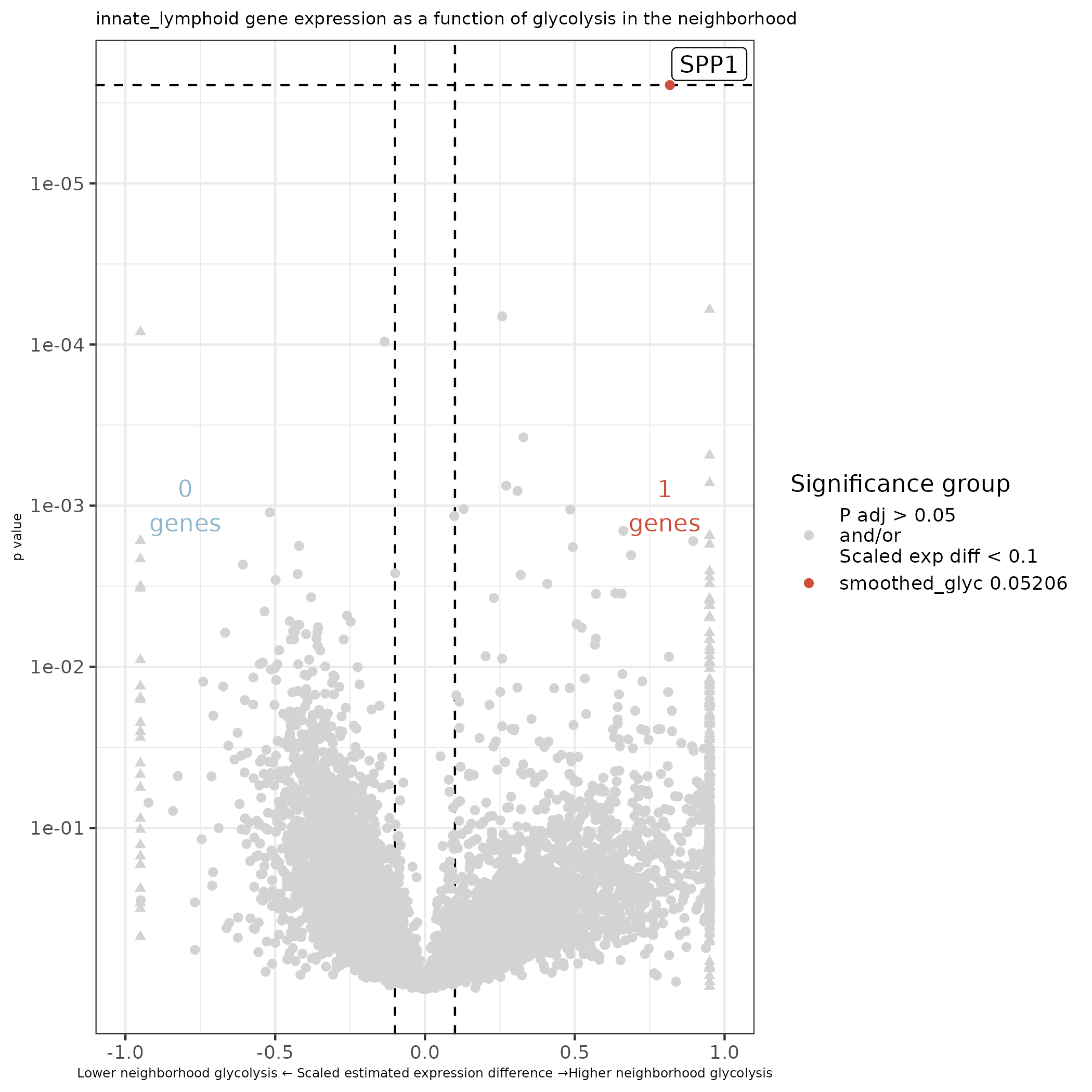
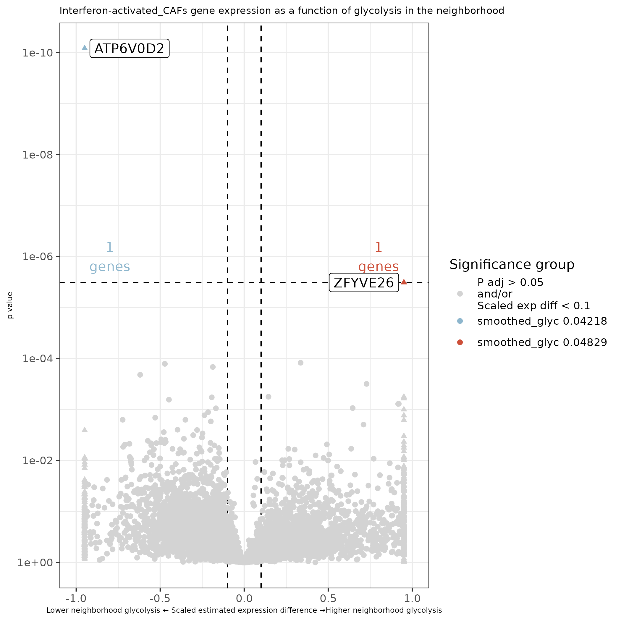
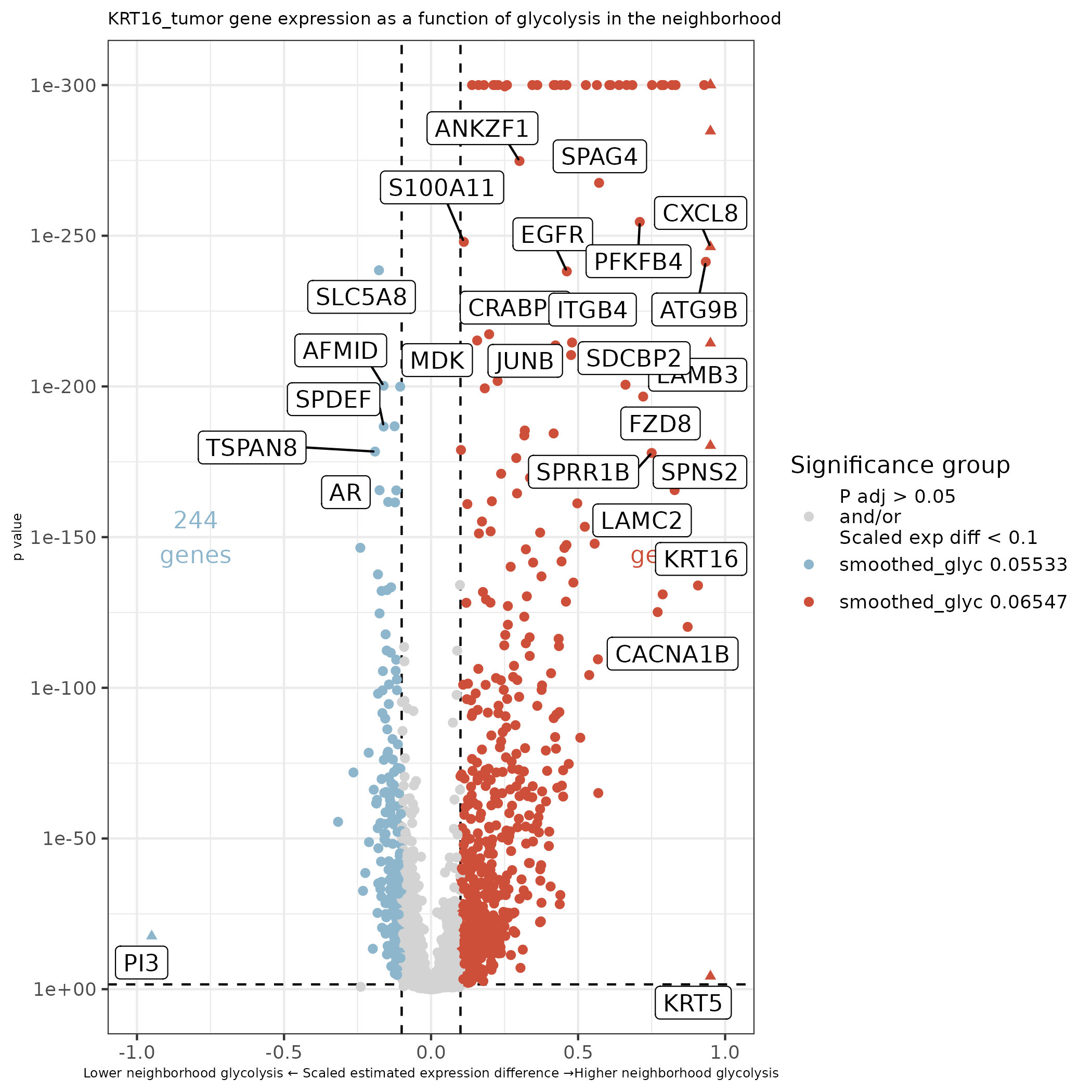
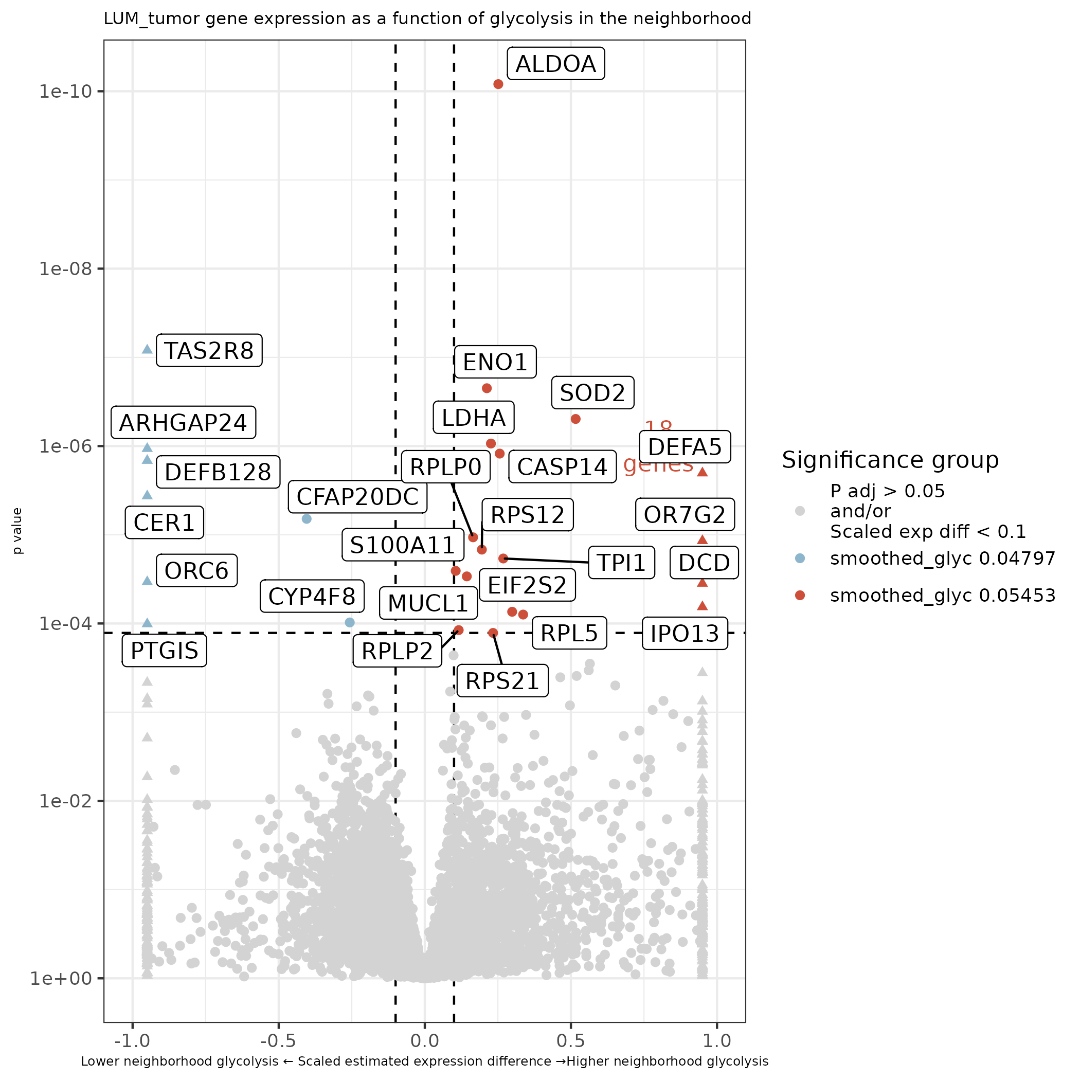
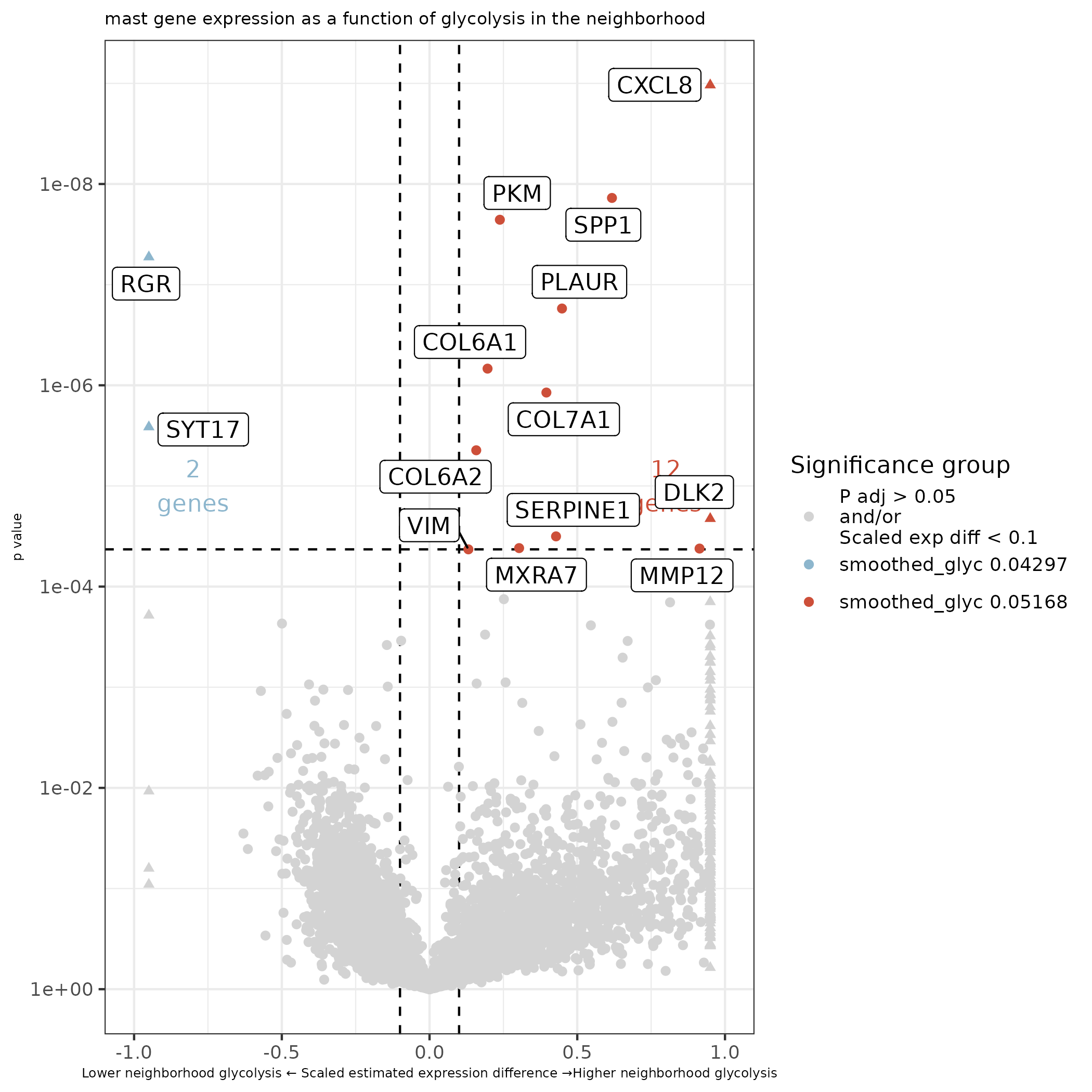
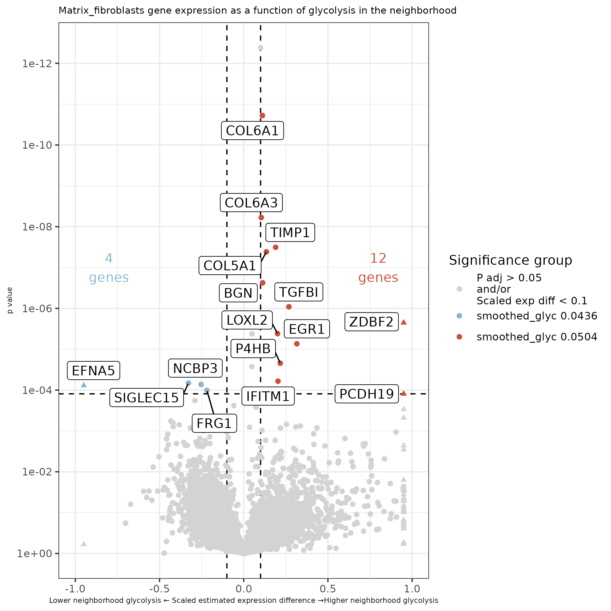
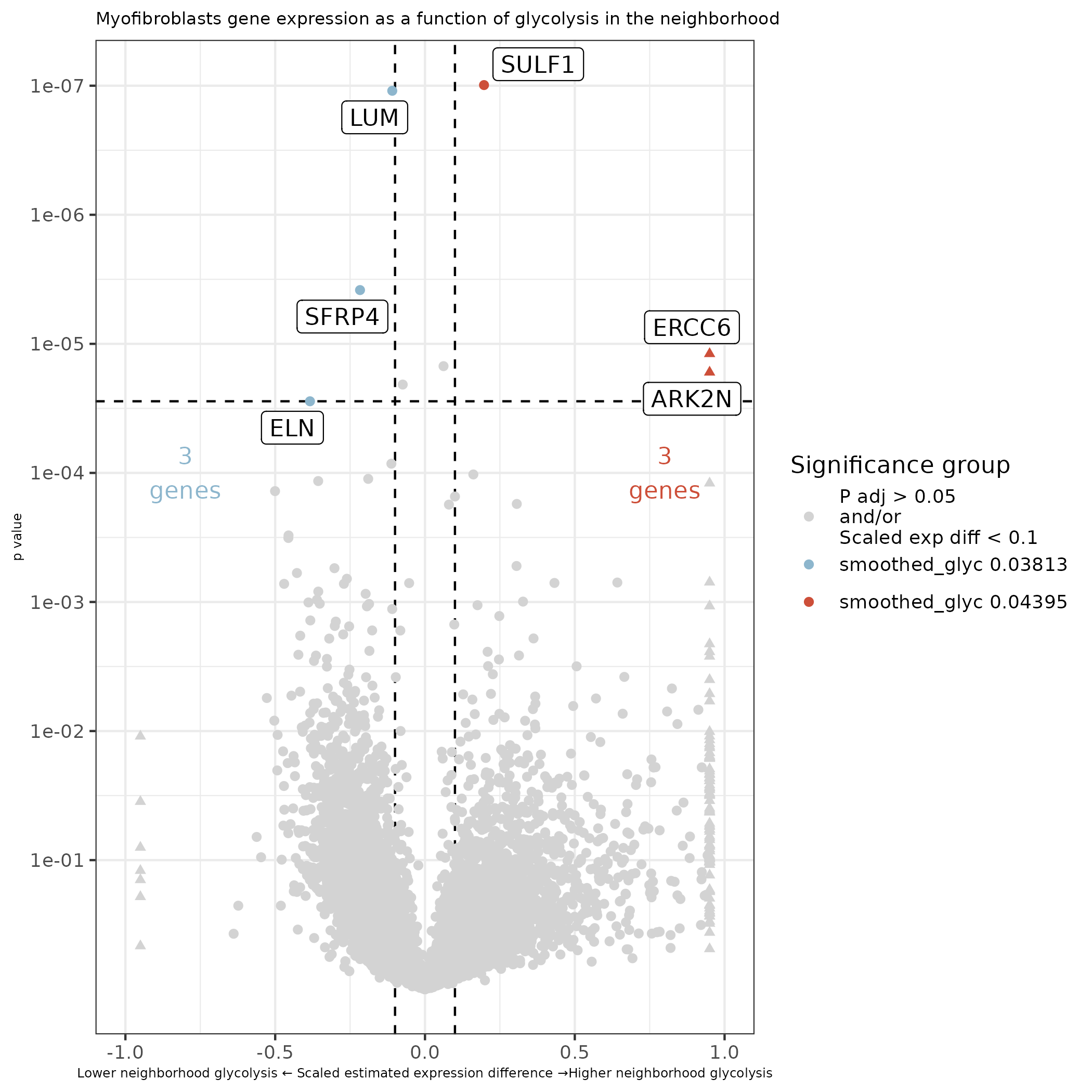
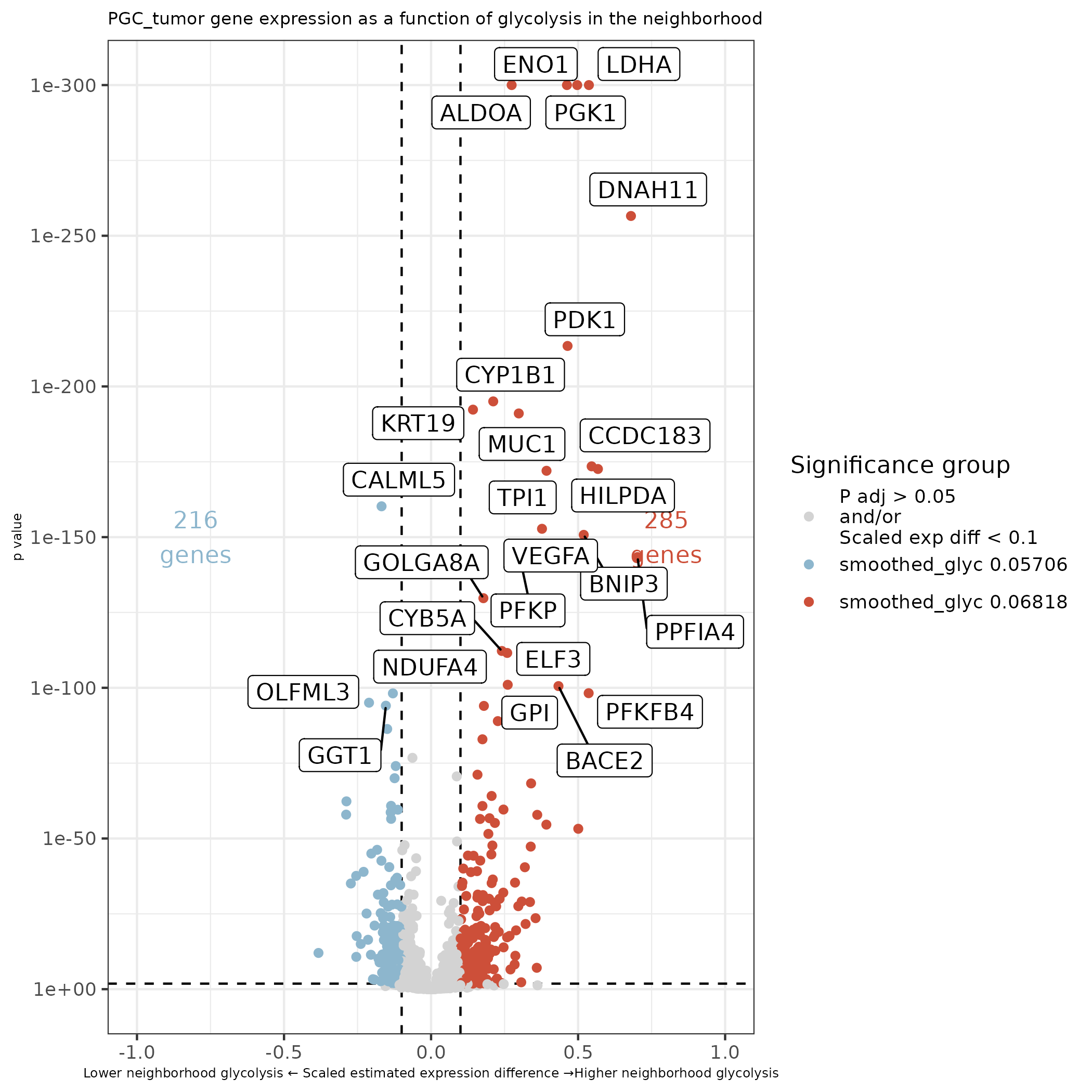
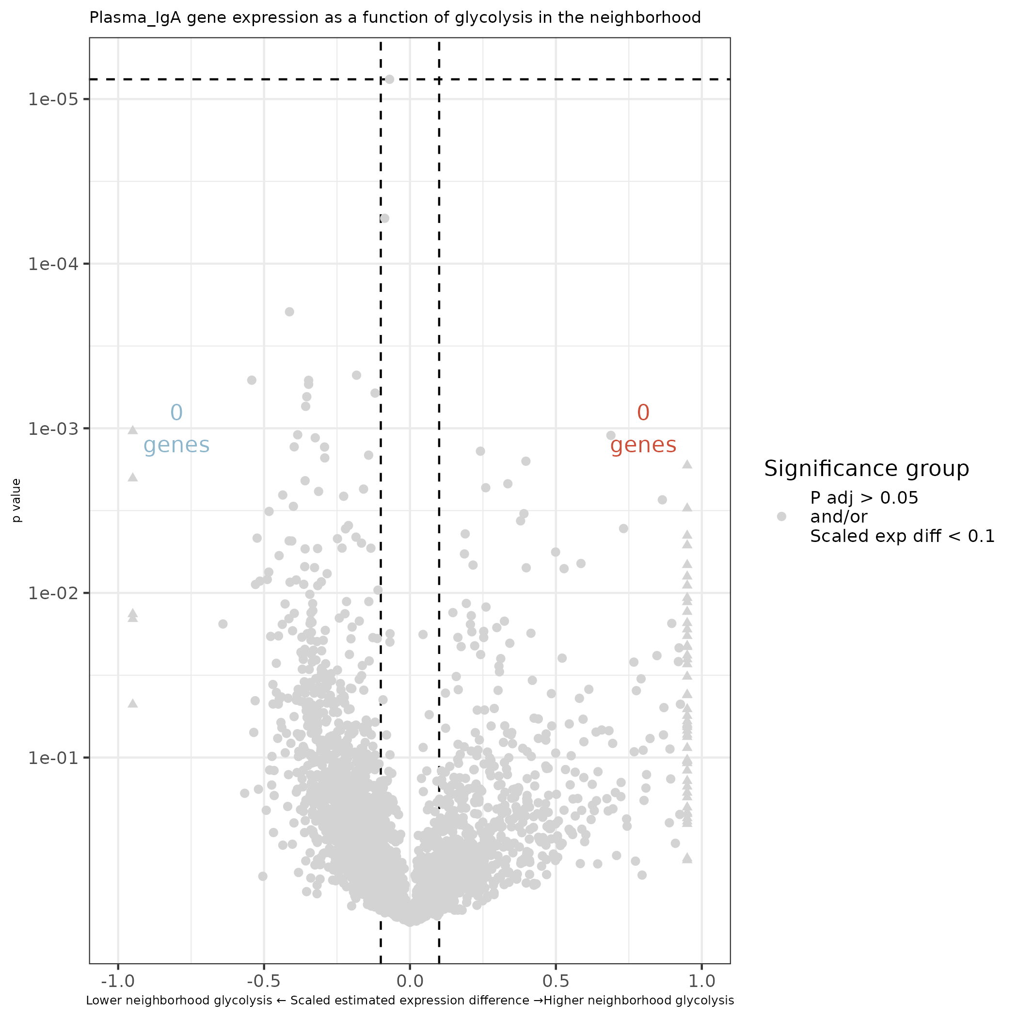
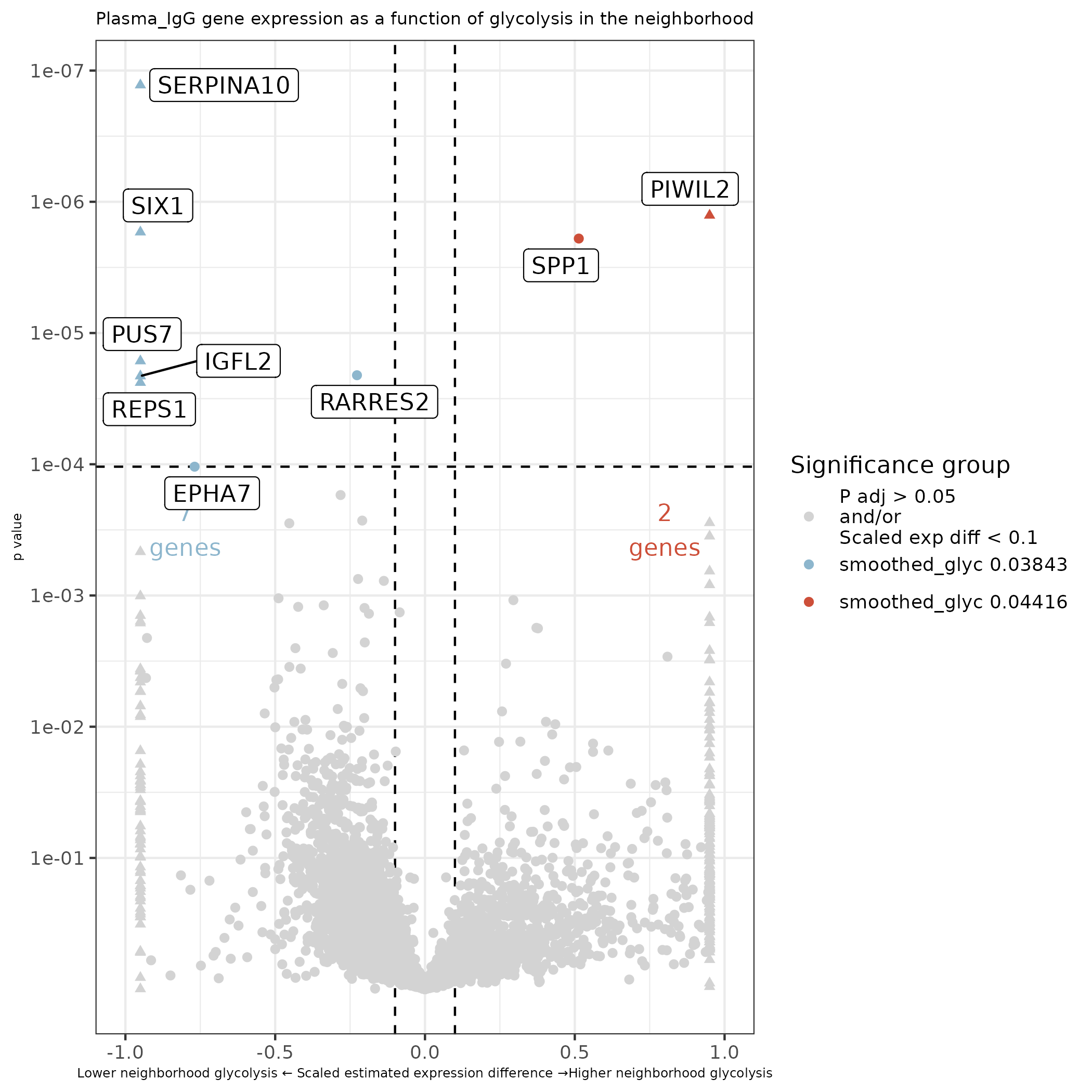
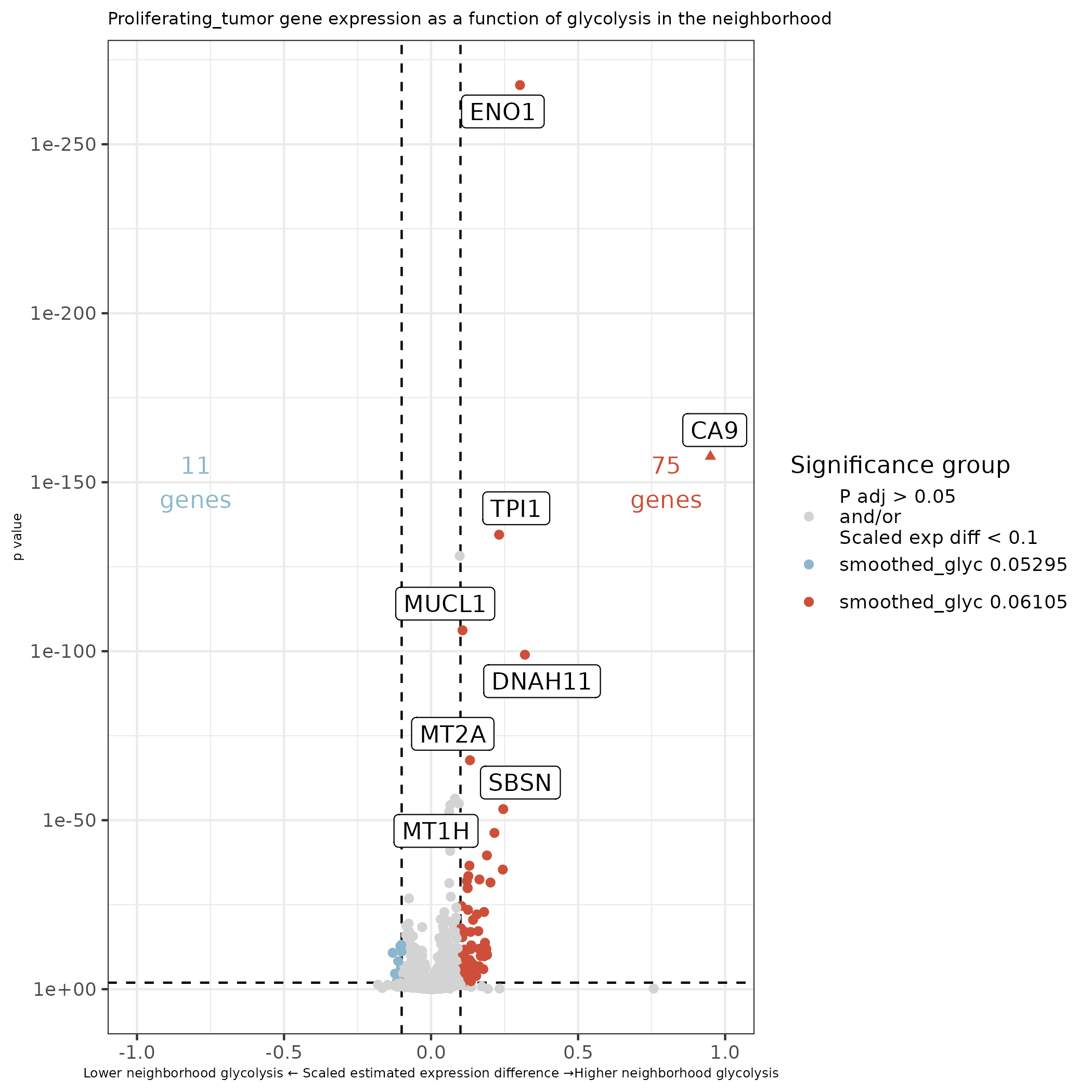
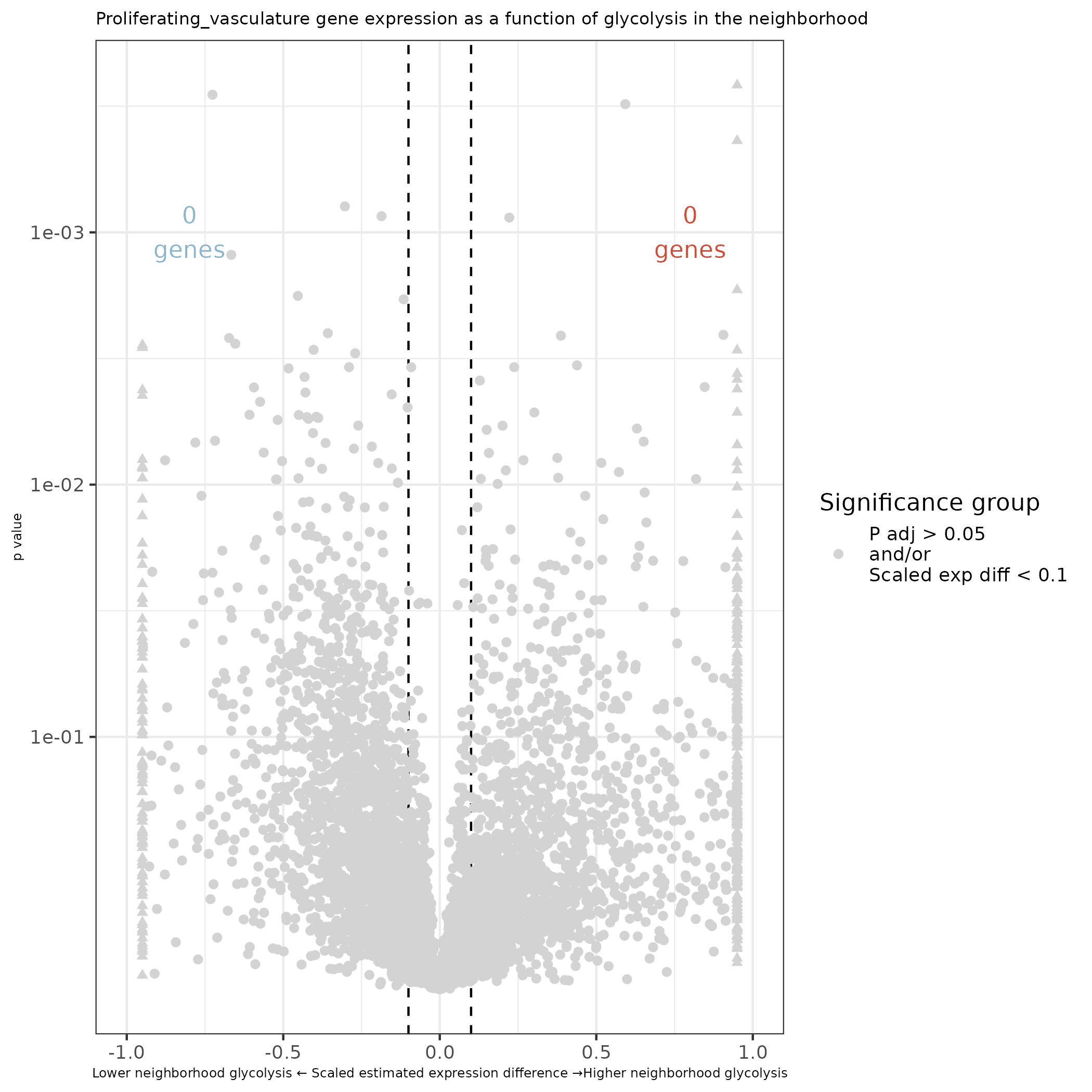
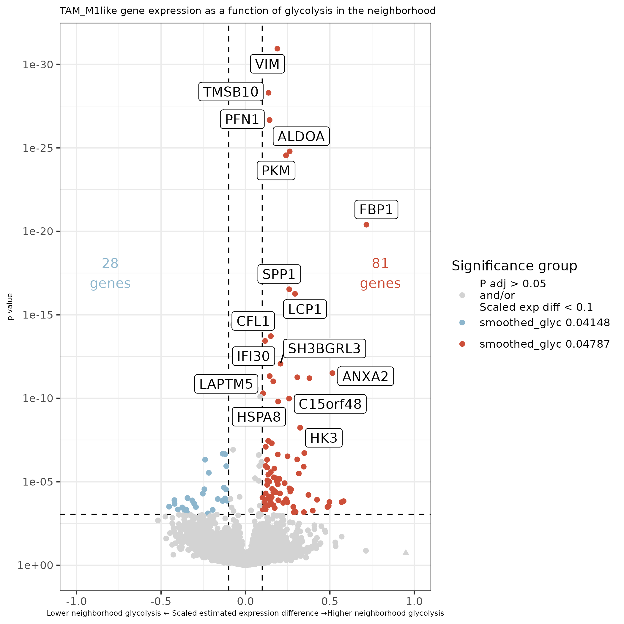
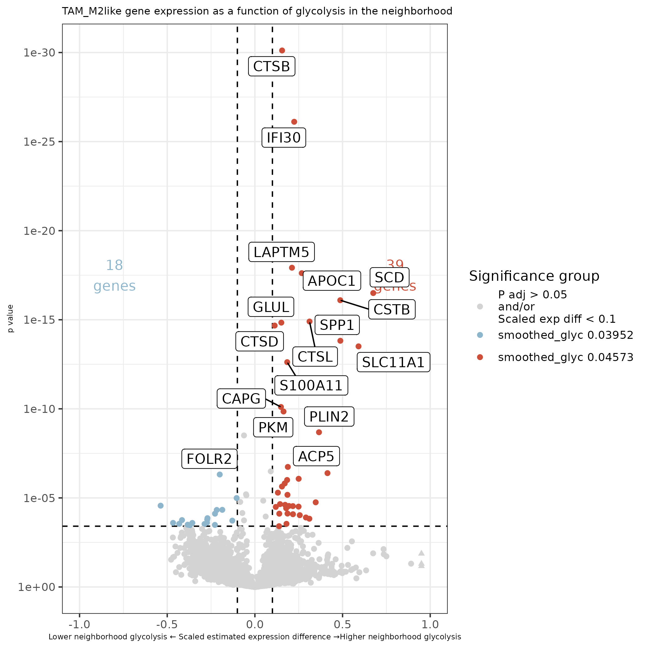
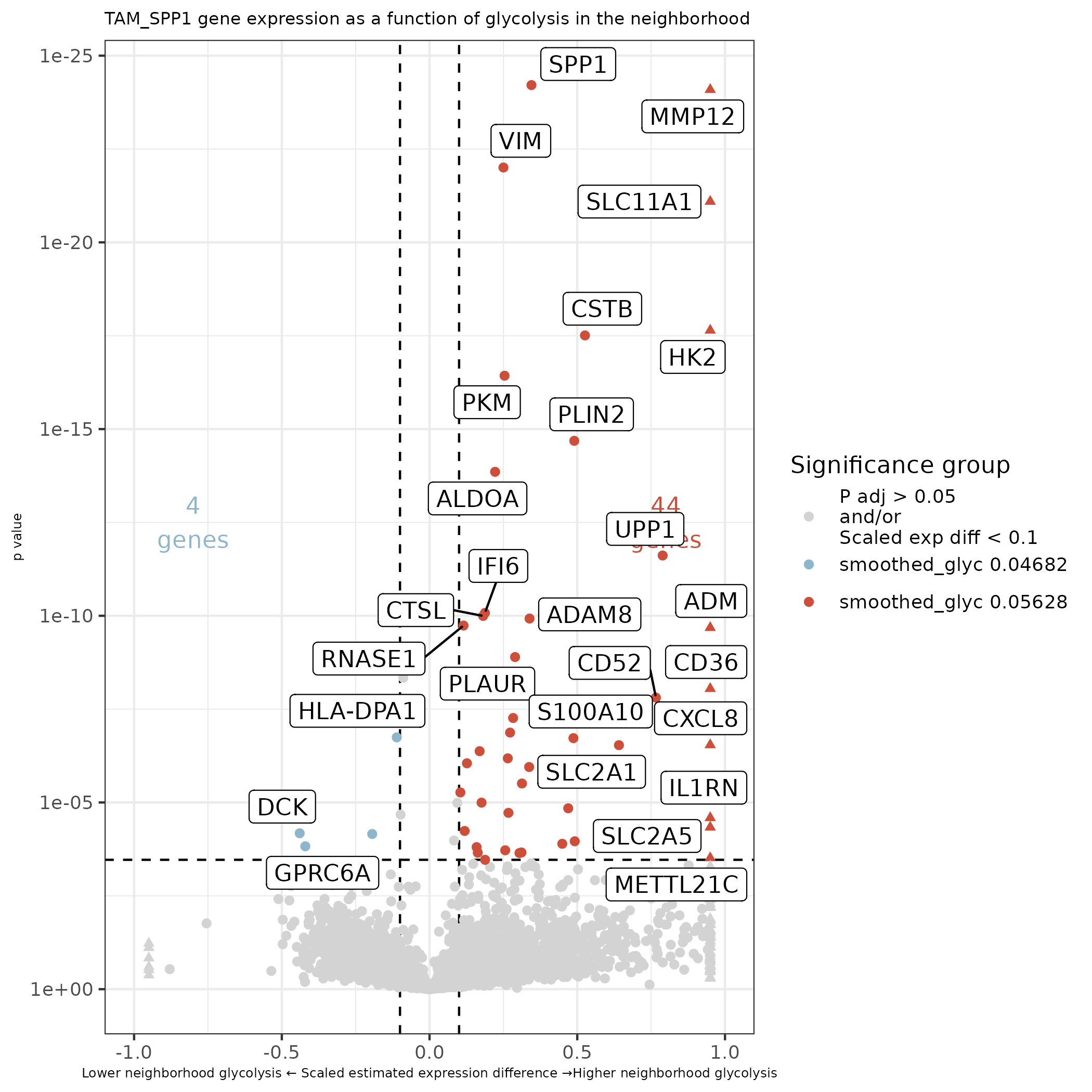
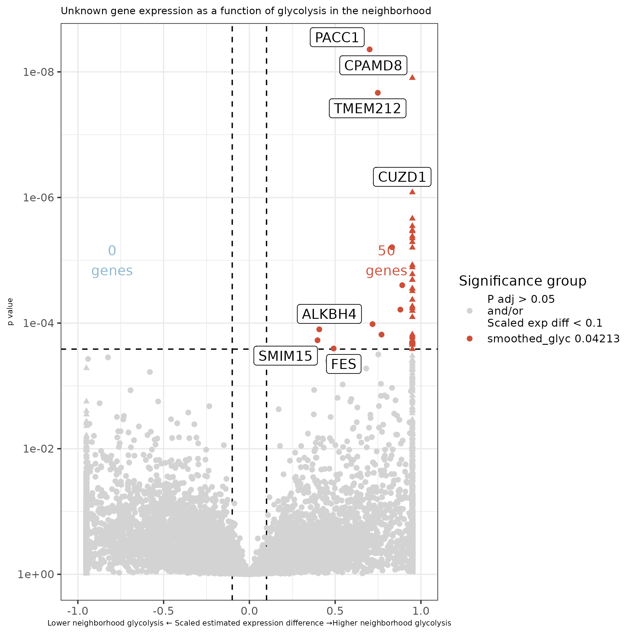
For every cell type, we make a volcano plot showing the estimated difference in expression between high and low glycolysis neighborhoods for each tested gene. Genes whose difference reached significance are colored and a subset are labeled. Also generate a table of DE results to be included as a supplementary table. Print each cell type to a separate sheet.

# Generate a list of pairwise DE results files
de_result_files <- dir(paste0(metabolism_dir, "/Data/"), pattern = "^ct_.*smoothedGlycolysis_de_obj_plusNicheNeighborTumor\\.rds$")

# Make a list of results to print to table
res_list <- list()

#de_res_list <- list()
for(de_file in de_result_files){
  de_obj <- readRDS(paste0(metabolism_dir, "/Data/", de_file))
  
  # Extract cell type
  ct <- gsub("ct_", "", gsub("_smoothedGlycolysis_de_obj_plusNicheNeighborTumor.rds", "", de_file))
  
  # Extract pairwise results, which correspond to difference between mean and 1SD of glycolysis score
  pairwise.df <- results(de_obj, "pairwise")$pairwise
  pairwise.df <- pairwise.df %>% filter(term == "smoothed_glyc") 
  
  # Adjust p-value
  pairwise.df$p.adj <- p.adjust(pairwise.df$p.value, method = "fdr") # Use fdr for padj
  res_list[[ct]] <- as.data.frame(pairwise.df)[,c("target", "estimate", "SE", "df", "t.ratio", "p.value",
                                                  "fold_change", "modelest_cpc_1", "modelest_cpc_2",
                                                  "term", "p.adj")]
  
  # Plot for each contrast, largely adapting smiDE volcano plot code
  for(contrast in unique(pairwise.df$contrast)){
    pairwise.df_i <- as.data.frame(pairwise.df)[which(pairwise.df$contrast == contrast),]

    # Extract comparison
    cc = pairwise.df_i$contrast[1]
    compv = compv <- strsplit(as.character(cc), "\\ vs.\\ ")[[1]]
    if(grepl(" [\\/-]\\ ", cc)) compv <- strsplit(as.character(cc), "\\ [\\/-]\\ ")[[1]]

    ## Plot with scaled estimates to adjust for expression levels

    # Large estimates disrupt scaling, so cap them and change the shape
    pairwise.df_i$scaled_estimate <- pairwise.df_i$estimate / pairwise.df_i$modelest_cpc_2
    pairwise.df_i$scaled_estimate_capped <- pmax(pmin(pairwise.df_i$scaled_estimate, 0.95), -0.95)
    pairwise.df_i$capped <- abs(pairwise.df_i$scaled_estimate) > 0.95

    # x labels
    xrng <- c((max(abs(pairwise.df_i$scaled_estimate_capped)) * -1),
              max(abs(pairwise.df_i$scaled_estimate_capped)))
    xrng <- pretty(xrng)

    # Set up y labels
    nDigits <- function(x) suppressWarnings(as.integer(strsplit(x = formatC(formatC(x = x, format="e"), format = "s"), split = "e")[[1]][2]))
    pairwise.df_i <- as.data.table(pairwise.df_i)
    bonf<- pairwise.df_i[,0.05/(uniqueN(target) * uniqueN(contrast))]
    max.y <- nDigits(min(pairwise.df_i[,min(p.value)+10^-300], signif(bonf / 2, 1)))

    ybrk <- 1 * 10^pretty( c(-1:(max.y)) )
    ylab <- ybrk

    # Add coloring
    est_cutoff = 0.1
    pairwise.df_i$sig_group = paste0("P adj > 0.05\nand/or\nScaled exp diff < ", est_cutoff)
    pairwise.df_i$sig_group[intersect(which(pairwise.df_i$p.adj < 0.05),
                                      which((pairwise.df_i$scaled_estimate) > est_cutoff))] <- compv[1]
    pairwise.df_i$sig_group[intersect(which(pairwise.df_i$p.adj < 0.05),
                                      which((pairwise.df_i$scaled_estimate) < -est_cutoff))] <- compv[2]
    my_cols = c("tomato3", "lightskyblue3", "lightgrey")
    names(my_cols) = c(compv[1],
                       compv[2],
                       paste0("P adj > 0.05\nand/or\nScaled exp diff < ", est_cutoff))

    # Set up yintercept for pval cutoff
    pval_cutoff_y <- pairwise.df %>% filter(p.adj < 0.05) %>% pull(p.value) %>% max()

    # Plot with top DE genes labeled
    ggplot(pairwise.df_i,
           aes(x = scaled_estimate_capped, y = p.value + 10^-300)) +
      geom_hline(yintercept = pval_cutoff_y, linetype = 2) +
      geom_vline(xintercept = est_cutoff, linetype = 2) +
      geom_vline(xintercept = -est_cutoff, linetype = 2) +
      geom_point(aes(color = sig_group, shape = capped)) +
      scale_shape_manual(values = c(`FALSE` = 19, `TRUE` = 17)) +
      scale_color_manual(values = my_cols, name = "Significance group") +
      scale_y_continuous(trans = smiDE:::change_axis_revlog_trans(base=10),
                         breaks = ybrk,
                         labels = formatC(ylab, format = "e", digits = 0)) +
      scale_x_continuous(breaks = xrng, limits = range(xrng)) +
      theme_bw() +
      ylab("p value") +
      xlab(paste0("Lower neighborhood glycolysis ", sprintf('\u2190'),
                  " Scaled estimated expression difference ",
                  sprintf('\u2192'), "Higher neighborhood glycolysis" )) +
      geom_text(data = pairwise.df[1,],
                aes(label = paste0(sum(pairwise.df_i$sig_group == compv[1]), "\ngenes"),
                    x = max(xrng)*0.8, y = sqrt(min(ybrk))),
                color = my_cols[[compv[1]]]) +
      geom_text(data = pairwise.df[1,],
                aes(label = paste0(sum(pairwise.df_i$sig_group == compv[2]), "\ngenes"),
                    x = min(xrng)*0.8, y = sqrt(min(ybrk))),
                color = my_cols[[compv[2]]]) +
      ggtitle(paste0(ct,
                     " gene expression as a function of glycolysis in the neighborhood")) +
      theme(plot.title = element_text(size = 8)) +
      theme(axis.title.x = element_text(size = 6)) +
      theme(axis.title.y = element_text(size = 6)) +
      geom_label_repel(data = pairwise.df_i %>% filter(!grepl("P adj", sig_group)),
                       aes(x = scaled_estimate_capped, y = p.value + 10^-300,
                           label = target)) +
      guides(shape = "none")
    ggsave(filename = paste0(metabolism_dir, "/Plots/", gsub("+", "", ct), "_volcano_GLYCneighborhoodDifferences_scaledEstDiff_", compv[1], "vs",
                             compv[2], "_withGeneLabels_v2.png"))
  }
}

# Print tables of results to excel file
xlsx_path <- file.path(metabolism_dir, "Data", "GlycolysisDE_by_celltype.xlsx")
writexl::write_xlsx(res_list, path = xlsx_path)

Volcano plot showing expression difference as a function of neighborhood glycolysis for all cell types:

bcell

cd4_naive

cd4_tcm

cd4_teff_th17

cd4_teff_th1

cd4_teff_th2

cd4_tem

cd4_treg

cd8_exhausted

cd8_naive

cd8_tcm

cd8_tem

dendritic

Endothelial_cells

HPD_tumor

Inflammatory_CAFs

innate_lymphoid

Interferon-activated_CAFs

KRT16_tumor

LUM_tumor

mast

Matrix_fibroblasts

Myofibroblasts

Necrotic_cells

neutrophil

nk

Pericytes

PGC_tumor

Plasma_IgA

Plasma_IgG

Proliferating_tumor

Proliferating_vasculature

TAM_M1like

TAM_M2like

TAM_SPP1

Unknown

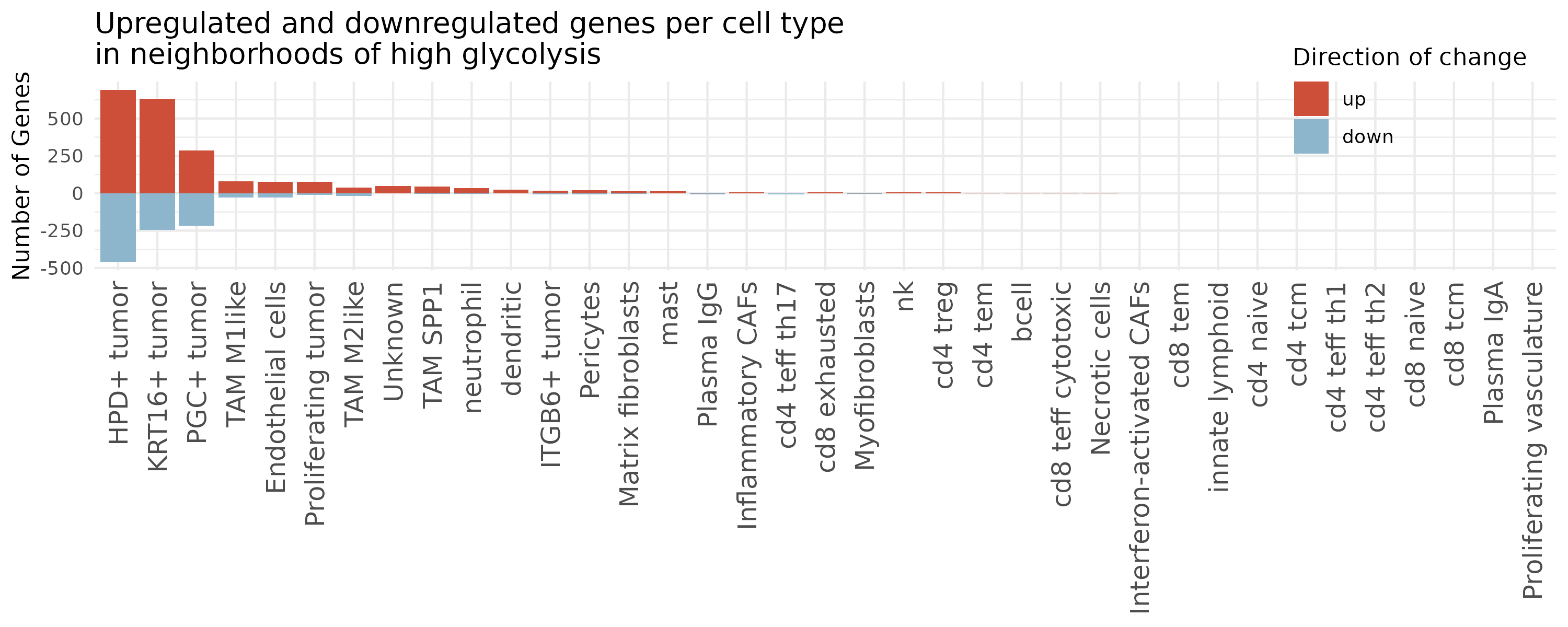
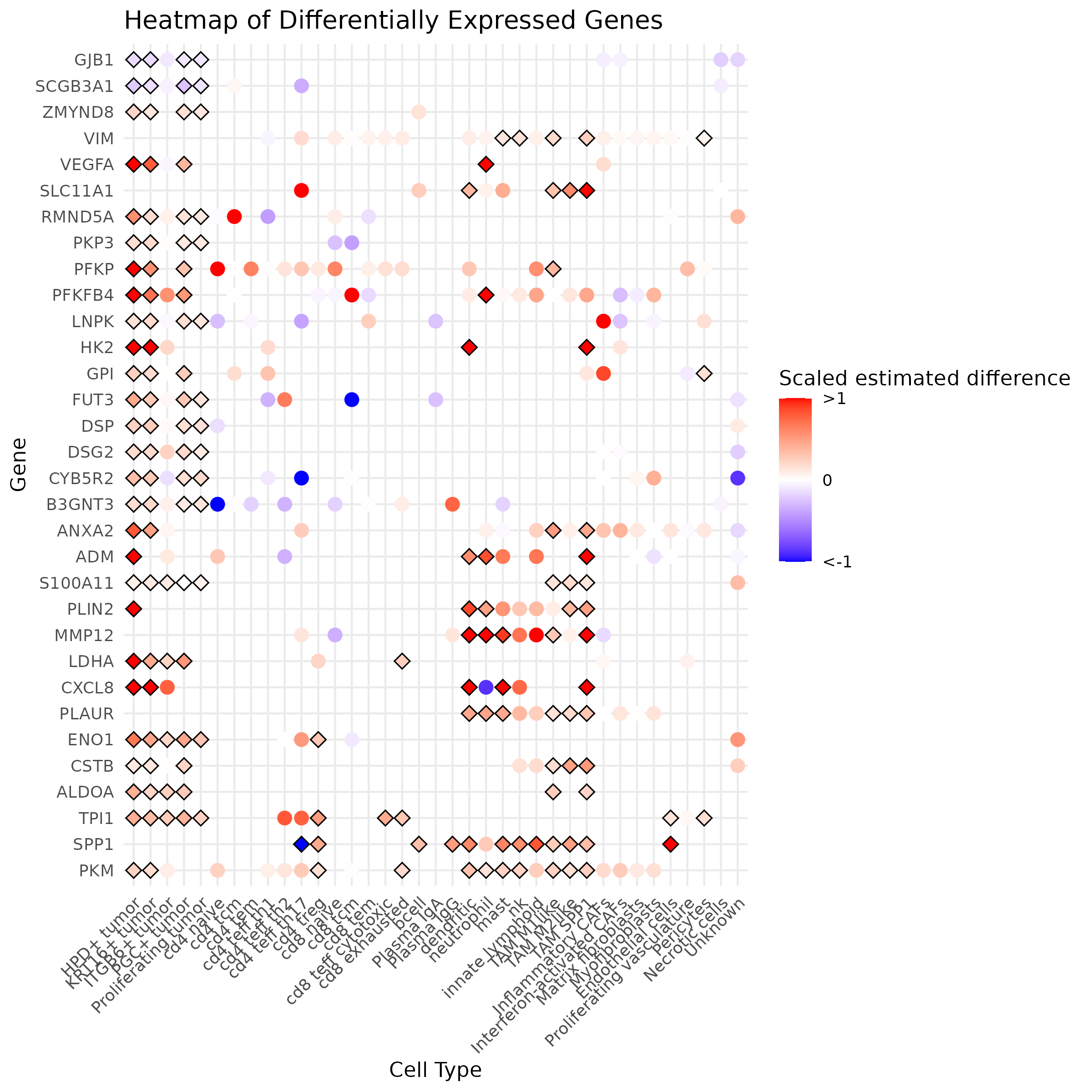
Additionally, we make summary plots to show results across all cell types. We generate a bar plot showing the number of genes called as significantly different across cell types and a heatmap showing most consistent genes across cell types.

# Generate a list of pairwise DE results
de_result_files <- dir(paste0(metabolism_dir, "/Data/"), pattern = "^ct_.*smoothedGlycolysis_de_obj_plusNicheNeighborTumor\\.rds$")

de_res_list <- list()
for(de_file in de_result_files){
  res <- readRDS(paste0(metabolism_dir, "/Data/", de_file))
  
  pairwise.df <- results(res)$pairwise
  pairwise.df <- pairwise.df %>% filter(term == "smoothed_glyc")
  
  # Extract cell type
  ct <- gsub("ct_", "", gsub("_smoothedGlycolysis_de_obj_plusNicheNeighborTumor.rds", "", de_file))
  
  # Convert underscore to space
  ct <- gsub("_", " ", ct)
  
  # Add a + for tumor cells except proliferating
  ct <- gsub(" tumor", "+ tumor", ct)
  ct <- gsub("Proliferating\\+", "Proliferating", ct)
  
  de_res_list[[ct]] <- pairwise.df
}

# Define a function to add the adjusted p-values
add_p_adj <- function(df) {
  df$p.adj <- p.adjust(df$p.value, method = "fdr") # Note the method used here
  return(df)
}

# Apply the function to each data frame in the list
de_res_list <- lapply(de_res_list, add_p_adj)


## Barplot showing the number of genes that are up or down regulated per cell type
# count significant genes
sig_genes <- list()

# Iterate through each data frame in the list
for (ct_name in names(de_res_list)) {
  df <- de_res_list[[ct_name]]
  
  # Filter for significant genes
  significant_genes <- df %>% filter(p.adj < 0.05) %>% filter(abs(estimate/modelest_cpc_2) > 0.1)
  
  # Count upregulated genes
  upregulated <- sum(significant_genes$estimate/significant_genes$modelest_cpc_2 > 0.1)
  
  # Count downregulated genes
  downregulated <- sum(significant_genes$estimate/significant_genes$modelest_cpc_2 < -0.1)
  
  # Count total genes evaluated
  tot_genes <- nrow(df)
  
  # Store the results in a data frame
  sig_genes[[ct_name]] <- data.frame(
    ct = ct_name,
    direction = c("up", "down"),
    nGenes = c(upregulated, downregulated),
    totGenes = tot_genes
  )
}

# Combine all results into a single data frame
sig_genes <- do.call(rbind, sig_genes)

# Order cell types by total genes changes
tot_genes_changed <- aggregate(sig_genes$nGenes ~ sig_genes$ct, FUN = "sum")
ct_order <- tot_genes_changed[order(tot_genes_changed[,2], decreasing = T),1]
sig_genes$ct <- factor(sig_genes$ct, levels = ct_order)

# Order direction for legend plotting
sig_genes$direction <- factor(sig_genes$direction, levels = c("up", "down"))

ggplot(sig_genes, aes(x = ct, y = ifelse(direction == "up", nGenes, -nGenes), fill = direction)) +
  geom_bar(stat = "identity") +
  scale_fill_manual(values = c("up" = "tomato3", "down" = "lightskyblue3")) +
  theme_minimal() +
  labs(title = "Upregulated and downregulated genes per cell type\nin neighborhoods of high glycolysis",
       #x = "Cell Type",
       y = "Number of Genes",
       fill = "Direction of change") +
  theme(axis.text.x = element_text(angle = 90, hjust = 1, vjust = 0.5, size = 12),
        axis.title.x = element_blank(),
        legend.position = c(0.9, 0.9))
ggsave(paste0(metabolism_dir, "/Plots/Barplot_sigGenes_glycolysisNeighborhood_byCT_scaledEstDiff_v2.png"),
       width = 10, height = 4, units = "in")

# Heatmap showing differences across multiple cell types
## Choose genes to show
# Initialize lists to store upregulated and downregulated genes
upregulated_genes <- list()
downregulated_genes <- list()

# Iterate through each data frame in the list
for (ct_name in names(de_res_list)) {
  df <- de_res_list[[ct_name]]
  
  # Filter for significant upregulated genes
  significant_upregulated <- df %>% filter(p.adj < 0.05) %>% filter(estimate/modelest_cpc_2 > 0.1)
  upregulated_genes[[ct_name]] <- significant_upregulated$target
  
  # Filter for significant downregulated genes
  significant_downregulated <- df %>% filter(p.adj < 0.05) %>% filter(estimate/modelest_cpc_2 < -0.1)
  downregulated_genes[[ct_name]] <- significant_downregulated$target
}

# Combine all upregulated and downregulated genes into single vectors
all_upregulated_genes <- unlist(upregulated_genes)
all_downregulated_genes <- unlist(downregulated_genes)

# Count the occurrences of each gene
up_gene_counts <- table(all_upregulated_genes)
down_gene_counts <- table(all_downregulated_genes)

# Sort genes by their counts in descending order
sorted_up_genes <- sort(up_gene_counts, decreasing = TRUE)
sorted_down_genes <- sort(down_gene_counts, decreasing = TRUE)

# Select genes that are significant in at least 4 cell types in a consistent direction
top_up_genes <- names(sorted_up_genes)[which(sorted_up_genes > 3)]
top_down_genes <- names(sorted_down_genes)[which(sorted_down_genes > 3)]

# Combine the top genes
top_genes <- unique(c(top_up_genes, rev(top_down_genes)))

## Make df of genes to show
# Initialize an empty data frame to store the heatmap data
heatmap_data <- data.frame()

# Iterate through each data frame in the list
for (ct_name in names(de_res_list)) {
  df <- de_res_list[[ct_name]]
  
  # Filter for the top genes
  df_top_genes <- df %>% filter(target %in% top_genes)
  
  # Add cell type information
  df_top_genes$ct <- ct_name
  
  # Append to the heatmap data frame
  heatmap_data <- rbind(heatmap_data, df_top_genes)
}

# Add a column for significance
heatmap_data$significant <- heatmap_data$p.adj < 0.05

# Set order of genes to have most consistently up -> most consistently down
heatmap_data$target <- factor(heatmap_data$target, levels = top_genes)

# Set order of cell types to align with other figures and be grouped by major type
heatmap_data$ct <- factor(heatmap_data$ct,
                          levels = gsub("_", " ", names(results_list$minor_cell_type_color_pal_manual)))

## Plot it

# Create the dot plot heatmap
ggplot(heatmap_data, aes(x = ct, y = target)) +
  geom_point(size = 0) +
  geom_point(data = heatmap_data %>% filter(significant == TRUE),
             aes(x = ct, y = target), color = "black", size = 4, shape = 18) +
  geom_point(data = heatmap_data, 
             aes(x = ct, y = target, color = estimate/modelest_cpc_2, shape = significant),
             size = 3) +
  scale_color_gradient2(low = "blue", mid = "white", high = "red", midpoint = 0,
                        limits = c(-1, 1),
                        oob = squish,
                        breaks = c(-1, 0, 1),
                        labels = c("<-1", "0", ">1")) +
  scale_size_manual(values = c(2,3), guide = "none") +
  scale_shape_manual(values = c('TRUE' = 18, 'FALSE' = 19), guide = "none") +
  theme_minimal() +
  labs(title = "Heatmap of Differentially Expressed Genes",
       x = "Cell Type",
       y = "Gene",
       color = "Scaled estimated difference") +
  theme(axis.text.x = element_text(angle = 45, hjust = 1))
ggsave(paste0(metabolism_dir, "/Plots/heatmap_ct_x_gene_mostDE_glycolysisNeighborhood_scaledEstDiff_v2.png"),
       width = 8, height = 8, units = "in")

Bar plot of the number of genes that are up / down regulated in each cell type as neighborhood glycolysis increases.

knitr::include_graphics(paste0(metabolism_dir, "/Plots/Barplot_sigGenes_glycolysisNeighborhood_byCT_scaledEstDiff_v2.png"))

Heatmap of the genes most consistently DE across cell types:

knitr::include_graphics(paste0(metabolism_dir,
                               "/Plots/heatmap_ct_x_gene_mostDE_glycolysisNeighborhood_scaledEstDiff_v2.png"))