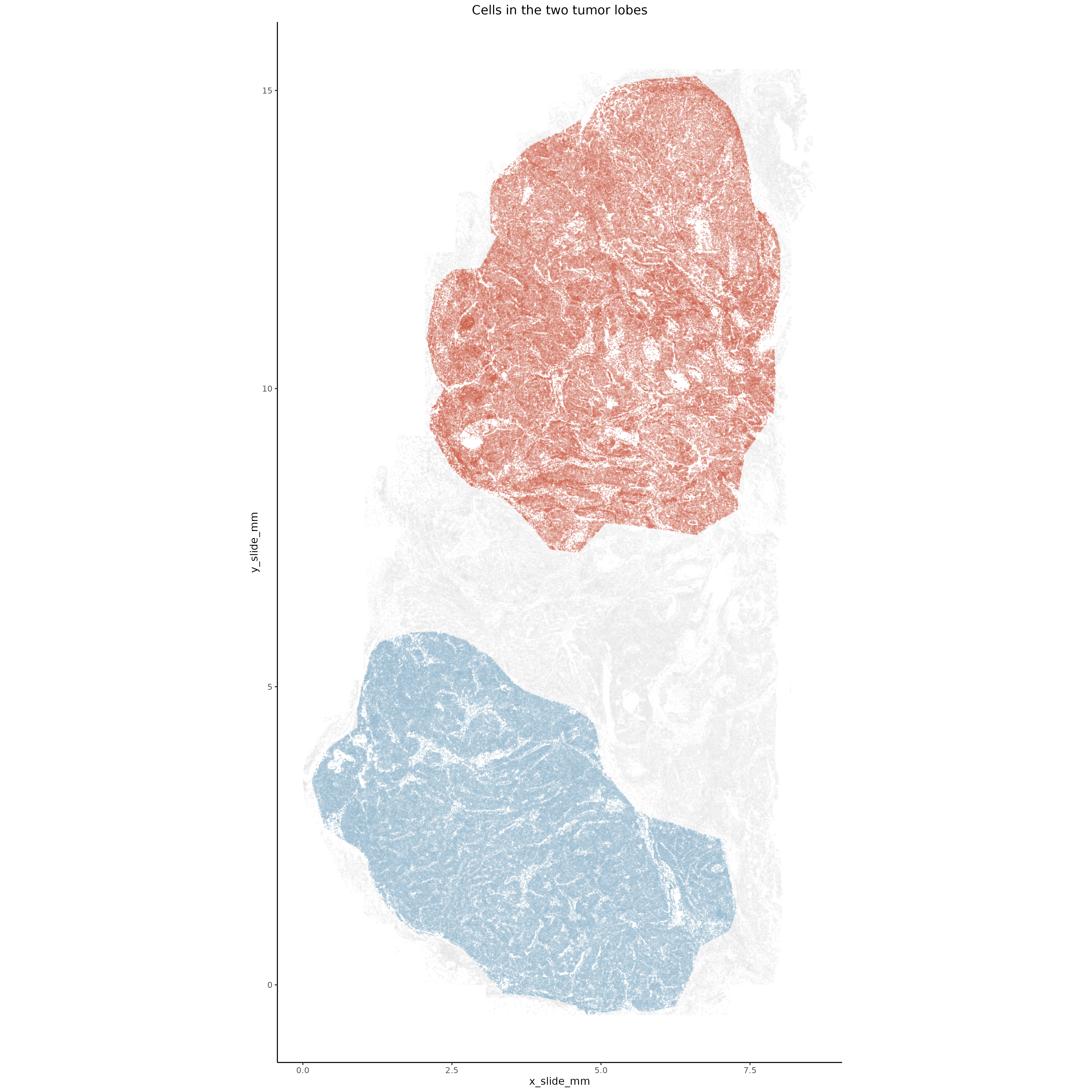
In this section we look to identify the major transcriptional differences between tumor cells in the lower dense lobe and tumor cells in the upper interdigitated lobe of the tumor.
4.1 Identify tumor lobes
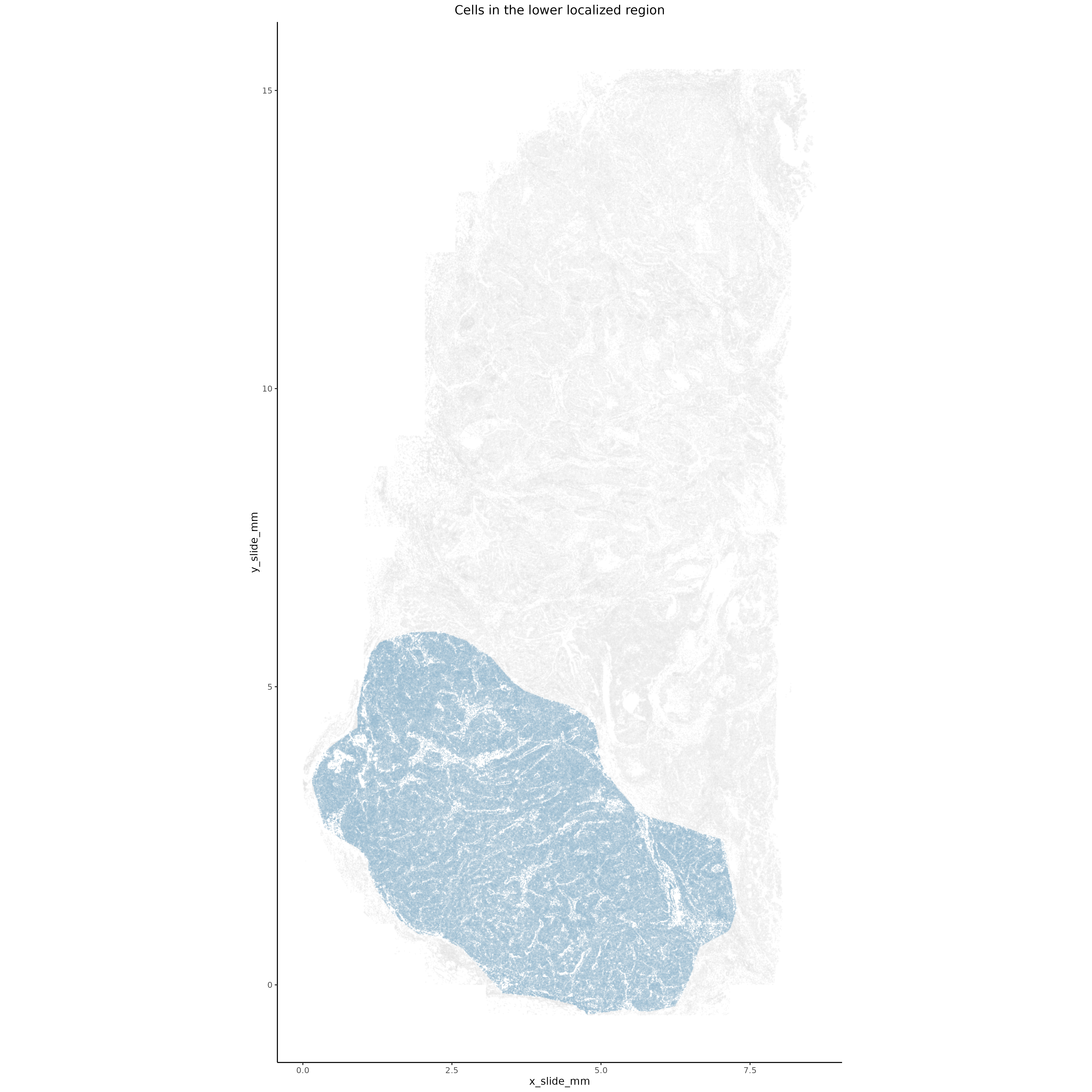
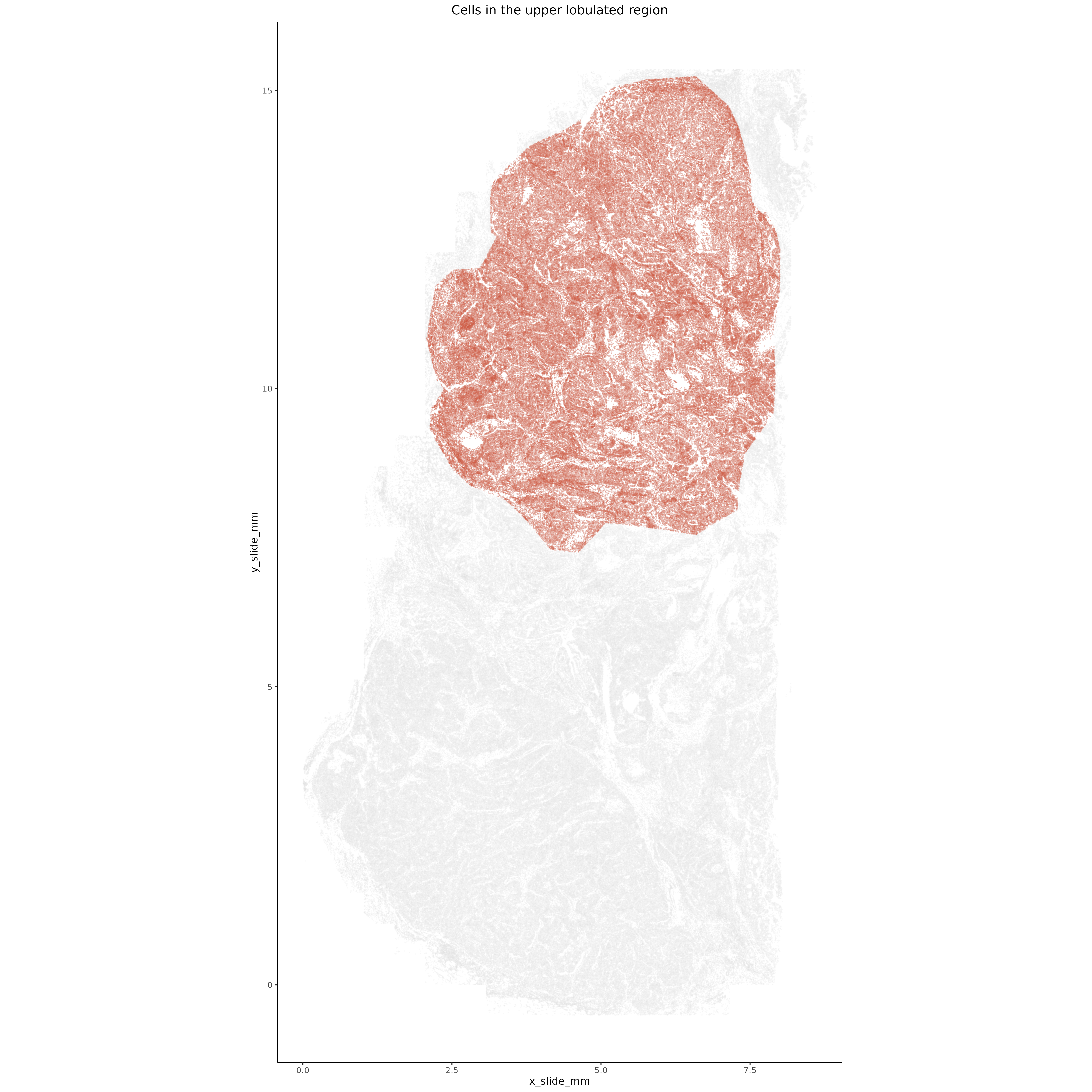
We first manually define the two main regions of the tumor - the bottom dense, localized lobe as well as the upper interdigitated lobe.
Manually draw a polygon around the lower localized tumor lobe.
Show the code
# if there's no seurat object, read it inif (!("seu.obj"%in%ls())){ seu.obj <-readRDS(results_list$seurat_file_postCellTyping)}if(is.null(results_list$lower_lobe_cells)){## Select outermost ring of cells to consider# Define a polygon selection function euclidean <-function(a, b) {sqrt(sum((a - b)^2)) } select_polygon <-function(distmin =0.01, max_points =40){message("Please select points to define a polygon. Click to the first point to stop. First point marker is largest.") lims <-par("usr") margins <-par("plt") calcX <-function(x, limitss = lims, mars = margins) limitss[1] + ((x-mars[1])/(1-(1-mars[2])-mars[1]))*(limitss[2]-limitss[1]) calcY <-function(y, limitss = lims, mars = margins) limitss[3] + ((y-mars[3])/(1-(1-mars[4])-mars[3]))*(limitss[4]-limitss[3]) calcXY <-function(z) c(calcX(z[1]), calcY(z[2]))# determine diagonal distance in the plotting coordinate frame diagonalDist <-euclidean(lims[c(1,3)], lims[c(2,4)])# select first and second point and third point pg <-matrix(c(0,0), nrow =1) pg[1, ] <-calcXY(unlist(grid::grid.locator(unit ="npc")))points(pg[1,1], pg[1,2], cex =1, pch =9, col ="magenta") pg <-rbind(pg, calcXY(unlist(grid::grid.locator(unit ="npc"))))points(pg[nrow(pg),1], pg[nrow(pg),2], cex =0.5, pch =9, col ="magenta") pg <-rbind(pg, calcXY(unlist(grid::grid.locator(unit ="npc"))))points(pg[nrow(pg),1], pg[nrow(pg),2], cex =0.5, pch =9, col ="magenta")#select additional points until a point is within the desired distance of the original point (or hit max_points limit)while(euclidean(pg[nrow(pg),], pg[1,]) > distmin*diagonalDist){ pg <-rbind(pg, calcXY(unlist(grid::grid.locator(unit ="npc"))))points(pg[nrow(pg),1], pg[nrow(pg),2], cex =0.5, pch =9, col ="magenta")if(nrow(pg) > max_points) {message("You reached the max allowed points.")break } }if(nrow(pg) >3) pg <- pg[1:(nrow(pg)-1),]polygon(pg[,1],pg[,2],col="#00000007",border="red")return(pg) }# Plot cells in bottom of tumorplot(seu.obj@meta.data$x_slide_mm, seu.obj@meta.data$y_slide_mm, cex =0.01, ylim =c(-0.5,6), asp=1, col =rgb(0,0,0,0.1))# Select outer tumor edge polygon manually pg_outer <-select_polygon()# which points are within the polygon idx_selected <- mgcv::in.out(pg_outer, as.matrix(seu.obj@meta.data[,c("x_slide_mm","y_slide_mm")] )) outer_cells <- seu.obj@meta.data$cell_id[idx_selected]# Add to results list results_list$lower_lobe_cells <- outer_cellssaveRDS(results_list, results_list_file)}
Manually draw a polygon around the upper interdigitated tumor lobe.
Show the code
if (!("seu.obj"%in%ls())){ seu.obj <-readRDS(results_list$seurat_file_postCellTyping)}if(is.null(results_list$upper_lobe_cells)){## Select outermost ring of cells to consider# Use function from above# Plot cells in upper region of slideplot(seu.obj@meta.data$x_slide_mm, seu.obj@meta.data$y_slide_mm, cex =0.01, ylim =c(6,16),asp=1, col =rgb(0,0,0,0.1))# Select outer tumor edge polygon manually pg_outer <-select_polygon()# which points are within the polygon idx_selected <- mgcv::in.out(pg_outer, as.matrix(seu.obj@meta.data[,c("x_slide_mm","y_slide_mm")] )) cells_in_upper <- seu.obj@meta.data$cell_id[idx_selected]# Add to results list results_list$upper_lobe_cells <- cells_in_uppersaveRDS(results_list, results_list_file)}
Plot cells in upper and lower lobes individually or simultaneously.
Show the code
if (!("seu.obj"%in%ls())){ seu.obj <-readRDS(results_list$seurat_file_postCellTyping)}# Plot upperggplot(seu.obj@meta.data,aes(x = x_slide_mm, y = y_slide_mm)) +geom_point(size =0.01, color ="light grey", alpha =0.1) +geom_point(data = seu.obj@meta.data[results_list$upper_lobe_cells,],aes(x = x_slide_mm, y = y_slide_mm),size =0.01, color ="tomato3", alpha =0.2) +theme_classic() +coord_fixed() +ggtitle("Cells in the upper lobulated region") +theme(plot.title =element_text(hjust =0.5))ggsave(filename =paste0(tumorDE_dir, "/Plots/XY_upperLobe.png"),width =16, height =16, units ="in")# Plot lowerggplot(seu.obj@meta.data,aes(x = x_slide_mm, y = y_slide_mm)) +geom_point(size =0.01, color ="light grey", alpha =0.1) +geom_point(data = seu.obj@meta.data[results_list$lower_lobe_cells,],aes(x = x_slide_mm, y = y_slide_mm),size =0.01, color ="lightskyblue3", alpha =0.2) +theme_classic() +coord_fixed() +ggtitle("Cells in the lower localized region") +theme(plot.title =element_text(hjust =0.5))ggsave(filename =paste0(tumorDE_dir, "/Plots/XY_lowerLobe.png"),width =16, height =16, units ="in")# Plot both togetherggplot(seu.obj@meta.data,aes(x = x_slide_mm, y = y_slide_mm)) +geom_point(size =0.01, color ="light grey", alpha =0.1) +geom_point(data = seu.obj@meta.data[results_list$lower_lobe_cells,],aes(x = x_slide_mm, y = y_slide_mm),size =0.01, color ="lightskyblue3", alpha =0.2) +geom_point(data = seu.obj@meta.data[results_list$upper_lobe_cells,],aes(x = x_slide_mm, y = y_slide_mm),size =0.01, color ="tomato3", alpha =0.2) +theme_classic() +coord_fixed() +ggtitle("Cells in the two tumor lobes") +theme(plot.title =element_text(hjust =0.5))ggsave(filename =paste0(tumorDE_dir, "/Plots/XY_bothLobes.png"),width =16, height =16, units ="in")
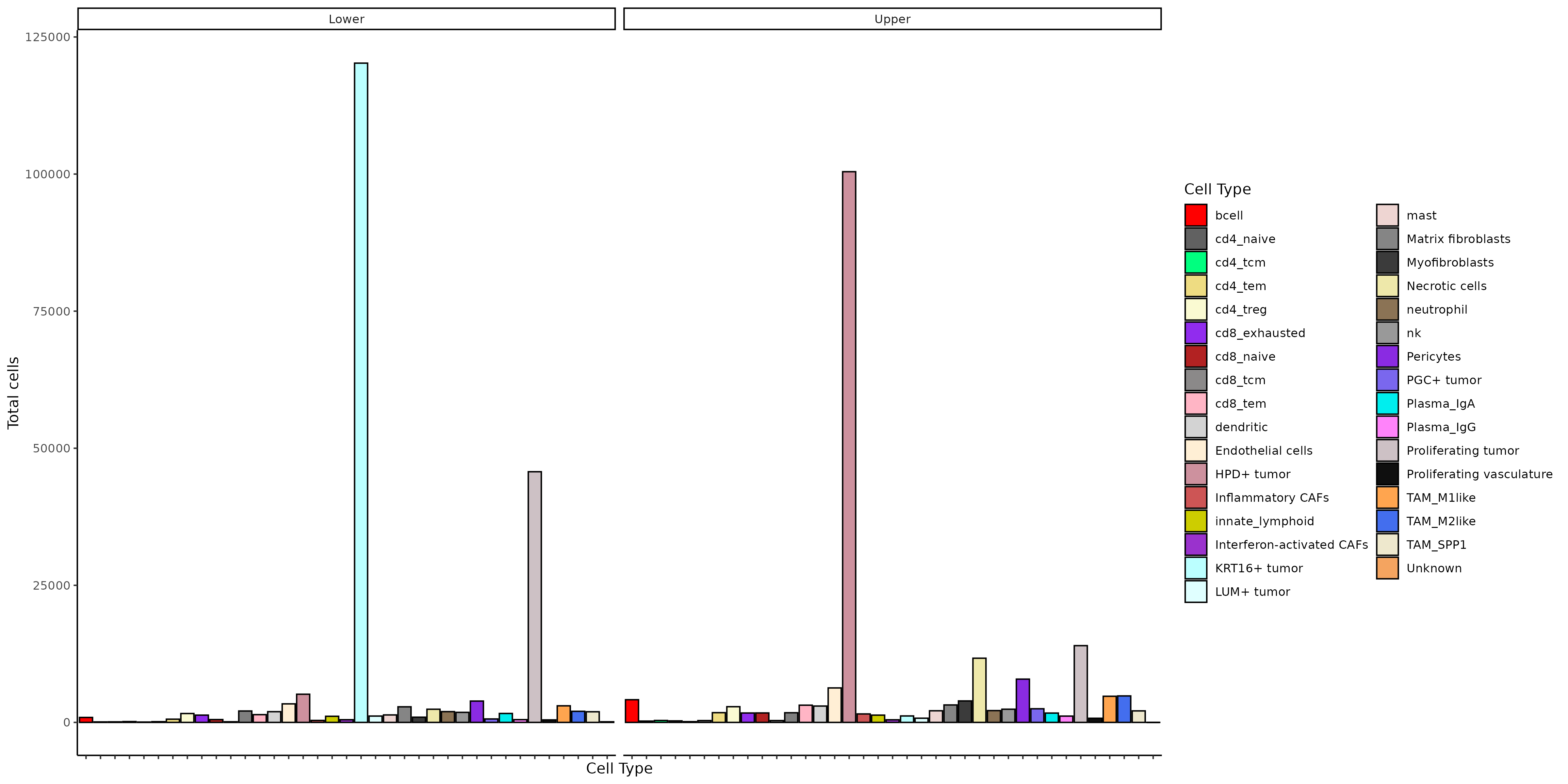
As a next basic step, we show cell type distributions in each lobe.
Show the code
if (!("seu.obj"%in%ls())){ seu.obj <-readRDS(results_list$seurat_file_postCellTyping)}# Isolate meta for plottingmeta <- seu.obj@meta.data# Add lobe assignmentsmeta$lobe <-"none"meta[results_list$upper_lobe_cells, "lobe"] <-"Upper"meta[results_list$lower_lobe_cells, "lobe"] <-"Lower"# Plot cell types by lobeggplot(meta[which(meta$lobe !="none"),], aes(x = minor_cell_type)) +geom_bar(aes(fill = minor_cell_type), color ="black") +scale_fill_manual(values = results_list$minor_cell_type_color_pal, name ="Cell Type") +xlab("Cell Type") +theme_classic() +theme(axis.text.x =element_blank()) +ylab("Total cells") +facet_wrap(~lobe)ggsave(filename =paste0(tumorDE_dir, "/Plots/Barplot_cellsPerCellType_byLobe.png"),width =16, height =8, unit ="in")
The major tumor type contributing to the top tumor are HPD+ tumor. In contrast, the major tumor type in the bottom tumor are KRT16+ and proliferating tumor.
We use differential expression to contrast tumor cells in the two lobes, using only genes that are more likely to be expressed in tumor cells than surrounding cells (ie are unlikely to be present simply due to tumor cells overlapping with non-tumor cells at their borders).
Show the code
if (!("seu.obj"%in%ls())){ seu.obj <-readRDS(results_list$seurat_file_postCellTyping)}# Isolate meta for plottingmeta <- seu.obj@meta.data# Add lobe assignmentsmeta$lobe <-"none"meta[results_list$upper_lobe_cells, "lobe"] <-"Upper"meta[results_list$lower_lobe_cells, "lobe"] <-"Lower"## Run DE between tumor lobes on tumor cells only# Pre-de find neighborspre_de_obj <-pre_de(metadata = meta,cell_type_metadata_colname ="major_cell_type",mm_radius =0.05,sdimx_colname ="x_slide_mm",sdimy_colname ="y_slide_mm",verbose =TRUE,adjacencies_only =TRUE)# Add total counts to metadata as DE expectsmeta$totalcounts = meta$nCount_RNA# Use overlap metric to identify genes to testoverlap_metrics <-smiDE::overlap_ratio_metric(assay_matrix = seu.obj@assays$RNA$data,metadata = meta,cluster_col ="major_cell_type",radius =0.05,#split_neighbors_by_colname = "Run_Tissue_name",sdimx_col ="x_slide_mm",sdimy_col ="y_slide_mm" )# Save overlap metricssaveRDS(overlap_metrics, file =paste0(tumorDE_dir, "/Data/overlap_metrics.rds"))# Only analyze genes with ratio less than or equal to 1analysis_genes <- overlap_metrics[major_cell_type=="Tumor"& ratio <=1]$target# DE test dependence on tumor lobede_obj <-smi_de(assay_matrix = seu.obj@assays$RNA@counts[analysis_genes,],metadata = meta[which(meta[,"major_cell_type"] =="Tumor"),],formula =~RankNorm(otherct_expr) + lobe +offset(log(totalcounts)),pre_de_obj = pre_de_obj,groupVar ="lobe",neighbor_expr_cell_type_metadata_colname ="major_cell_type",neighbor_expr_totalcount_normalize =TRUE,neighbor_expr_totalcount_scalefactor =NULL,family ="nbinom2",targets = analysis_genes,nCores =20)# Save objectssaveRDS(pre_de_obj, file =paste0(tumorDE_dir, "/Data/pre_de_obj.rds"))saveRDS(de_obj, file =paste0(tumorDE_dir, "/Data/de_obj_tumorGenes.rds"))
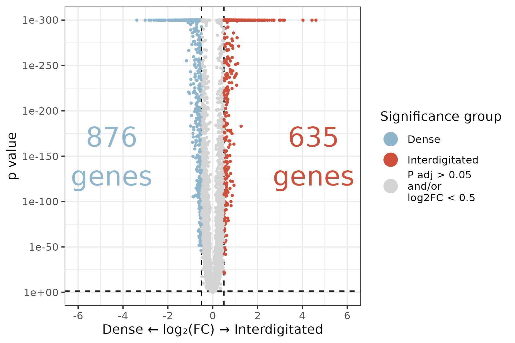
With the major differences between tumor cells in the two lobes, we first generate a volcano plot to visually demonstrate the vast differences between these two lobes. Also save these results to a table.
Show the code
# Read in DE objectde_obj <-readRDS(paste0(tumorDE_dir, "/Data/de_obj_tumorGenes.rds"))# Extract pairwise results, invasive vs localized lobepairwise.df <-results(de_obj, "pairwise")$pairwisepairwise.df <- pairwise.df %>%filter(term =="lobe") %>%filter(contrast =="Lower / Upper")# Convert terminology to Dense / Interdigitatedpairwise.df$contrast <-gsub("Lower / Upper", "Dense / Interdigitated", pairwise.df$contrast)# Adjust p-valuepairwise.df$p.adj <-p.adjust(pairwise.df$p.value, method ="fdr")# Save pairwise results to a table to be included as supplementary information.write.csv(as.data.frame(pairwise.df)[,c(setdiff(colnames(pairwise.df), c("df", "null", "fold_change")))],file =paste0(tumorDE_dir, "/Data/TumorLobeDE_table.csv"),row.names =FALSE)# Plot it, partially following smiDE volcano code# Ensure that the lower lobe is plotted on the left to align with tissue image# Extract comparisoncc = pairwise.df$contrast[1]compv = compv <-strsplit(as.character(cc), "\\ vs.\\ ")[[1]]if(grepl(" [\\/-]\\ ", cc)) compv <-strsplit(as.character(cc), "\\ [\\/-]\\ ")[[1]]# x labelsxrng <- pairwise.df[!is.na(log2(fold_change)),c(min(-log2(fold_change)),max(-log2(fold_change)))]xrng <-c(-max(abs(xrng)), max(abs(xrng)))xrng <-pretty(xrng)# Set up y labelsnDigits <-function(x) suppressWarnings(as.integer(strsplit(x =formatC(formatC(x = x, format="e"), format ="s"), split ="e")[[1]][2]))bonf<- pairwise.df[,0.05/(uniqueN(target) *uniqueN(contrast))]max.y <-nDigits(min(pairwise.df[,min(p.value)+10^-300], signif(bonf /2, 1)))ybrk <-1*10^pretty( c(-1:(max.y)) )ylab <- ybrk# Add coloringfc_cutoff =0.5pairwise.df$sig_group =paste0("P adj > 0.05\nand/or\nlog2FC < ", fc_cutoff)pairwise.df$sig_group[intersect(which(pairwise.df$p.adj <0.05),which(log2(pairwise.df$fold_change) > fc_cutoff))] <- compv[1]pairwise.df$sig_group[intersect(which(pairwise.df$p.adj <0.05),which(log2(pairwise.df$fold_change) <-fc_cutoff))] <- compv[2]my_cols =c("tomato3", "lightskyblue3", "lightgrey")names(my_cols) =c("Interdigitated","Dense",paste0("P adj > 0.05\nand/or\nlog2FC < ", fc_cutoff))ggplot(pairwise.df,aes(x =-log2(fold_change), y = p.value +10^-300)) +# Negative log fold change switches the L/R order of upper / lowergeom_hline(yintercept =0.05, linetype =2) +geom_vline(xintercept = fc_cutoff, linetype =2) +geom_vline(xintercept =-fc_cutoff, linetype =2) +geom_point(aes(color = sig_group), size =0.6) +scale_color_manual(values = my_cols, name ="Significance group") +scale_y_continuous(trans = smiDE:::change_axis_revlog_trans(base=10),breaks = ybrk,labels =formatC(ylab, format ="e", digits =0)) +scale_x_continuous(breaks = xrng, limits =range(xrng)) +theme_bw() +ylab("p value") +xlab(paste0(compv[1], " ", sprintf('\u2190'), " log", sprintf('\u2082'), "(FC) ", sprintf('\u2192'), " ", compv[2]) ) +# Compv 1 and 2 are switched in order from usual to account for L/R switch of categoriesgeom_text(data = pairwise.df[1,], aes(label =paste0(sum(pairwise.df$sig_group =="Interdigitated"), "\ngenes"), x =min(abs(max(xrng)), abs(min(xrng)))*0.75, y =sqrt(min(ybrk))),color = my_cols[["Interdigitated"]], size =8) +geom_text(data = pairwise.df[1,], aes(label =paste0(sum(pairwise.df$sig_group =="Dense"), "\ngenes"), x =-min(abs(max(xrng)), abs(min(xrng)))*0.75, y =sqrt(min(ybrk))),color = my_cols[["Dense"]], size =8) +guides(color =guide_legend(override.aes =list(size =5)))ggsave(filename =paste0(tumorDE_dir, "/Plots/volcano_lobeDifferences_tumorGenes.png"),width =6, height =4, units ="in")
Warning in attr(x, "align"): 'xfun::attr()' is deprecated.
Use 'xfun::attr2()' instead.
See help("Deprecated")
Warning in attr(x, "format"): 'xfun::attr()' is deprecated.
Use 'xfun::attr2()' instead.
See help("Deprecated")
Description
FoldEnrichment
qvalue
R-HSA-71291
Metabolism of amino acids and derivatives
3.449887
0.0000000
R-HSA-8978868
Fatty acid metabolism
4.204344
0.0000000
R-HSA-1428517
Aerobic respiration and respiratory electron transport
3.207833
0.0000009
R-HSA-2408522
Selenoamino acid metabolism
4.477243
0.0000017
R-HSA-156902
Peptide chain elongation
4.792308
0.0000111
R-HSA-192823
Viral mRNA Translation
4.792308
0.0000111
R-HSA-9633012
Response of EIF2AK4 (GCN2) to amino acid deficiency
4.477243
0.0000117
R-HSA-156842
Eukaryotic Translation Elongation
4.588380
0.0000130
R-HSA-2408557
Selenocysteine synthesis
4.588380
0.0000130
R-HSA-72764
Eukaryotic Translation Termination
4.588380
0.0000130
R-HSA-975956
Nonsense Mediated Decay (NMD) independent of the Exon Junction Complex (EJC)
4.492788
0.0000156
R-HSA-72613
Eukaryotic Translation Initiation
4.017081
0.0000156
R-HSA-72737
Cap-dependent Translation Initiation
4.017081
0.0000156
R-HSA-9711097
Cellular response to starvation
3.555178
0.0000156
R-HSA-9837999
Mitochondrial protein degradation
4.401099
0.0000162
R-HSA-156827
L13a-mediated translational silencing of Ceruloplasmin expression
4.077489
0.0000222
R-HSA-1799339
SRP-dependent cotranslational protein targeting to membrane
4.041405
0.0000226
R-HSA-72706
GTP hydrolysis and joining of the 60S ribosomal subunit
4.041405
0.0000226
R-HSA-72689
Formation of a pool of free 40S subunits
4.228507
0.0000232
R-HSA-927802
Nonsense-Mediated Decay (NMD)
3.936886
0.0000290
R-HSA-975957
Nonsense Mediated Decay (NMD) enhanced by the Exon Junction Complex (EJC)
3.936886
0.0000290
R-HSA-8868773
rRNA processing in the nucleus and cytosol
3.122590
0.0000325
R-HSA-6791226
Major pathway of rRNA processing in the nucleolus and cytosol
3.154237
0.0000444
R-HSA-611105
Respiratory electron transport
3.350892
0.0000448
R-HSA-9010553
Regulation of expression of SLITs and ROBOs
3.350892
0.0000448
R-HSA-72312
rRNA processing
2.970268
0.0000682
R-HSA-376176
Signaling by ROBO receptors
2.955849
0.0000717
R-HSA-211859
Biological oxidations
2.844287
0.0000858
R-HSA-168273
Influenza Viral RNA Transcription and Replication
3.357932
0.0002202
R-HSA-156580
Phase II - Conjugation of compounds
3.657087
0.0002303
R-HSA-1655829
Regulation of cholesterol biosynthesis by SREBP (SREBF)
5.074208
0.0002601
R-HSA-72766
Translation
2.432840
0.0003960
R-HSA-168255
Influenza Infection
3.070381
0.0004021
R-HSA-2426168
Activation of gene expression by SREBF (SREBP)
5.436652
0.0008942
R-HSA-9865881
Complex III assembly
6.830665
0.0014179
R-HSA-191273
Cholesterol biosynthesis
6.577677
0.0017984
R-HSA-9609507
Protein localization
2.784626
0.0022374
R-HSA-200425
Carnitine shuttle
9.061086
0.0037464
R-HSA-1268020
Mitochondrial protein import
3.903237
0.0055081
R-HSA-9711123
Cellular response to chemical stress
2.422361
0.0083602
R-HSA-8957322
Metabolism of steroids
2.635952
0.0093358
R-HSA-74182
Ketone body metabolism
10.148416
0.0101201
R-HSA-2142753
Arachidonate metabolism
3.870159
0.0110064
R-HSA-75105
Fatty acyl-CoA biosynthesis
4.799927
0.0116904
R-HSA-9735869
SARS-CoV-1 modulates host translation machinery
4.799927
0.0116904
R-HSA-72662
Activation of the mRNA upon binding of the cap-binding complex and eIFs, and subsequent binding to 43S
3.805656
0.0116904
R-HSA-8963691
Phenylalanine and tyrosine metabolism
9.225833
0.0137704
R-HSA-9754678
SARS-CoV-2 modulates host translation machinery
3.979771
0.0167732
R-HSA-163210
Formation of ATP by chemiosmotic coupling
6.342760
0.0183869
R-HSA-72695
Formation of the ternary complex, and subsequently, the 43S complex
3.903237
0.0183869
R-HSA-163685
Integration of energy metabolism
2.819005
0.0220411
R-HSA-5218921
VEGFR2 mediated cell proliferation
6.040724
0.0221412
R-HSA-2046104
alpha-linolenic (omega3) and linoleic (omega6) acid metabolism
7.806474
0.0243856
R-HSA-2046106
alpha-linolenic acid (ALA) metabolism
7.806474
0.0243856
R-HSA-8949613
Cristae formation
4.612916
0.0302987
R-HSA-5628897
TP53 Regulates Metabolic Genes
3.020362
0.0304101
R-HSA-71240
Tryptophan catabolism
7.248869
0.0313439
R-HSA-5579029
Metabolic disorders of biological oxidation enzymes
4.477243
0.0337472
R-HSA-72649
Translation initiation complex formation
3.440141
0.0355114
R-HSA-72702
Ribosomal scanning and start codon recognition
3.440141
0.0355114
R-HSA-9759194
Nuclear events mediated by NFE2L2
2.916212
0.0364330
R-HSA-156590
Glutathione conjugation
4.228507
0.0427836
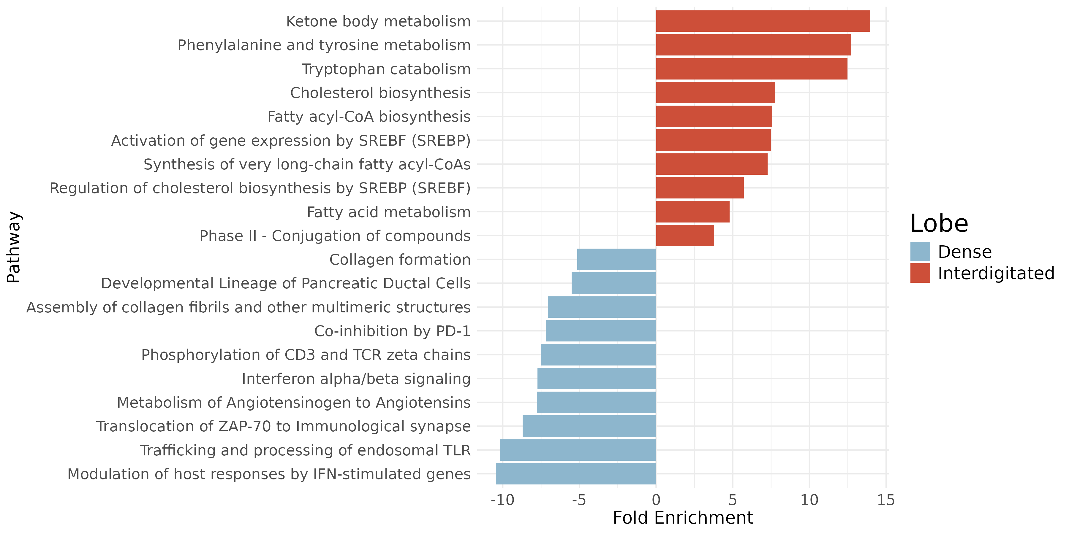
Plot top pathways enriched as a bar plot.
Show the code
# Read in pathway resultspathway_res <-readRDS(file =paste0(tumorDE_dir, "/Data/pathwayEnrichmentResults_tumorGenes.rds"))# Merge top enriched pathwaysenrich_paths <-rbind(pathway_res$upper_genes@result, pathway_res$lower_genes@result)enrich_paths$direction <-c(rep("upper", nrow(pathway_res$upper_genes@result)),rep("lower", nrow(pathway_res$lower_genes@result)))# Filter data frame for p.adjust < 0.1df_filtered <- enrich_paths %>%filter(p.adjust <0.1)# Add a column for bar length based on directiondf_filtered <- df_filtered %>%mutate(bar_length =ifelse(direction =="upper", FoldEnrichment, -FoldEnrichment),color =ifelse(direction =="upper", -log10(p.adjust), -log10(p.adjust)))# Arrange data frame by Fold Enrichment from highest to lowestdf_filtered <- df_filtered %>%arrange(desc(bar_length))# Select top 5 in each direction by absolute bar lengthdf_top <- df_filtered %>%mutate(abs_length =abs(bar_length)) %>%group_by(direction) %>%slice_max(order_by = abs_length, n =5, with_ties =FALSE) %>%ungroup()# Convert lobe terminologydf_top$direction <-gsub("lower", "Dense", df_top$direction)df_top$direction <-gsub("upper", "Interdigitated", df_top$direction)# Custom shorten a few pathway names for plottingdf_top$Description <- dplyr::recode(df_top$Description,"Modulation of host responses by IFN-stimulated genes"="*Modulation by IFN","Deposition of new CENPA-containing nucleosomes at the centromere"="*Nucleosome deposition","alpha-linolenic (omega3) and linoleic (omega6) acid metabolism"="*ALA (omega3) and LA (omega6) metabolism")# Create the plotggplot(df_top, aes(x =reorder(Description, bar_length), y = bar_length, fill = direction)) +geom_bar(stat ="identity") +scale_fill_manual(values =c("Dense"="lightskyblue3", "Interdigitated"="tomato3")) +coord_flip() +theme_minimal() +labs(y ="Fold Enrichment", x ="Pathway", fill ="Lobe") +theme(axis.text.y =element_text(size =12),axis.text.x =element_text(size =12),axis.title.y =element_text(size =14),axis.title.x =element_text(size =14),legend.text =element_text(size =14),legend.title =element_text(size =20))ggsave(filename =paste0(tumorDE_dir, "/Plots/barplot_pathwayEnrichmentByLobe_tumorGenes.png"),width =12, height =4, units ="in")