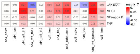
In this section, we explore the immune landscape of the tumor, highlighting immune-related pathways that vary regionally, immune cell distribution, and changes in immune cell transcriptomes based on environment.
5.1 Immune marker genes
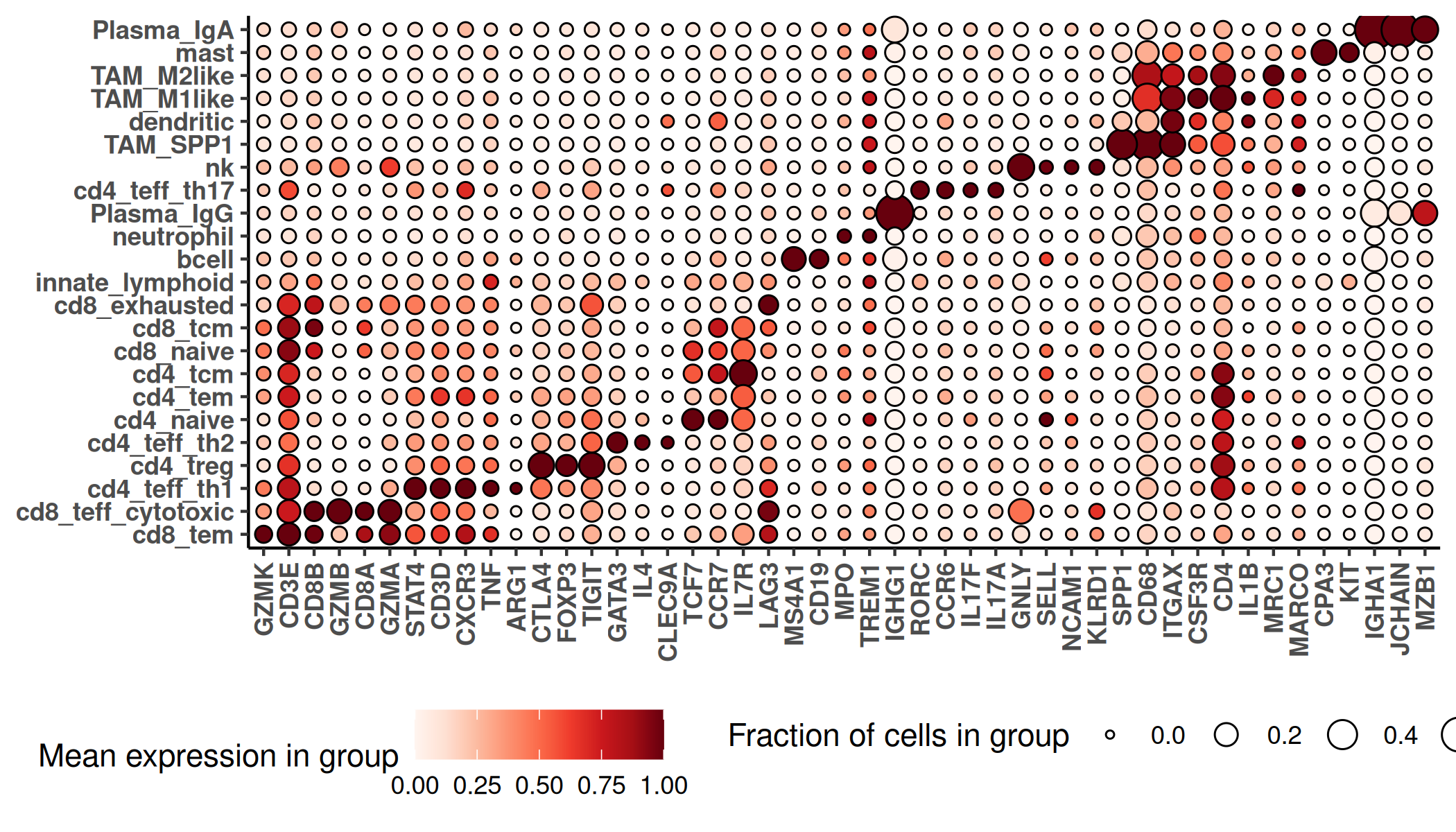
We generate a marker gene heatmap for the immune cells specifically, using canonical marker genes for each cell type.
Show the code
if(!("seu.obj"%in%ls())){ seu.obj <-readRDS(results_list$seurat_file_postCellTyping)}## prepare data for marker gene heatmap:idx =which(seu.obj$major_cell_type %in%c("dendritic", "Macrophage", "mast", "neutrophil", "bcell", "innate_lymphoid", "nk", "Plasma", "Tcell"))ct ="minor_cell_type"fc_subclus_ctl_gran <-clusterwise_foldchange_metrics(seu.obj[["RNA"]]@counts[,idx] ,metadata = seu.obj@meta.data[idx,] ,cluster_column = ct)# subtract background from the mean per-cluster expression profiles:# Extract neg countsneg_counts <- seu.obj@assays$negprobes$countsfor (name inunique(seu.obj@meta.data[idx,ct])) {if(is.na(name)){next} isthiscelltype <- seu.obj@meta.data[idx,ct] == name meannegthiscelltype <-mean(Matrix::colMeans(neg_counts[,idx][, isthiscelltype])) idy = fc_subclus_ctl_gran$cluster == name fc_subclus_ctl_gran$cluster_expr[idy] <- fc_subclus_ctl_gran$cluster_expr[idy] - meannegthiscelltype}fc_subclus_ctl_gran$cluster_expr[which(fc_subclus_ctl_gran$cluster_expr <0)] <-0# Establish one or two well known markers for each cell typegoi <-c('CD3D', 'CD3E', 'CD19', 'MS4A1', 'CD68', 'MARCO', 'ITGAX', 'CLEC9A','KIT', 'CPA3', 'MPO', 'CSF3R', 'NCAM1', 'KLRD1', 'IL7R', 'RORC','JCHAIN', 'MZB1', 'CD8B', 'CD8A', 'CD4', 'CCR7', 'TCF7','CCR6', 'CXCR3', 'STAT4', 'CXCR3', 'GATA3', 'IL4', 'IL17A', 'IL17F','FOXP3', 'CTLA4', 'TCF7', 'IL7R', 'GZMK', 'GZMA', 'SELL', 'GZMB','GNLY', 'LAG3', 'TIGIT', 'SPP1', 'TREM1', 'ARG1', 'MRC1', 'IL1B','TNF', 'IGHA1', 'IGHG1')hm_goi <-marker_heatmap(fc_subclus_ctl_gran, topn =0, featsuse =unique(goi)) +theme(legend.direction ="horizontal", # Arrange items within a legend horizontallylegend.position ="bottom", # Place the entire legend box at the bottomlegend.box ="horizontal"# Arrange multiple legend boxes horizontally )png(filename =paste0(immNeigh_dir, "/Plots/heatmap_", ct, "_immuneOnly_negRemoved_selectIndexMarkers.png"),width =7, height =4, units ="in", res =300)print(hm_goi)dev.off()
Heatmap of immune cells showing well-known markers.
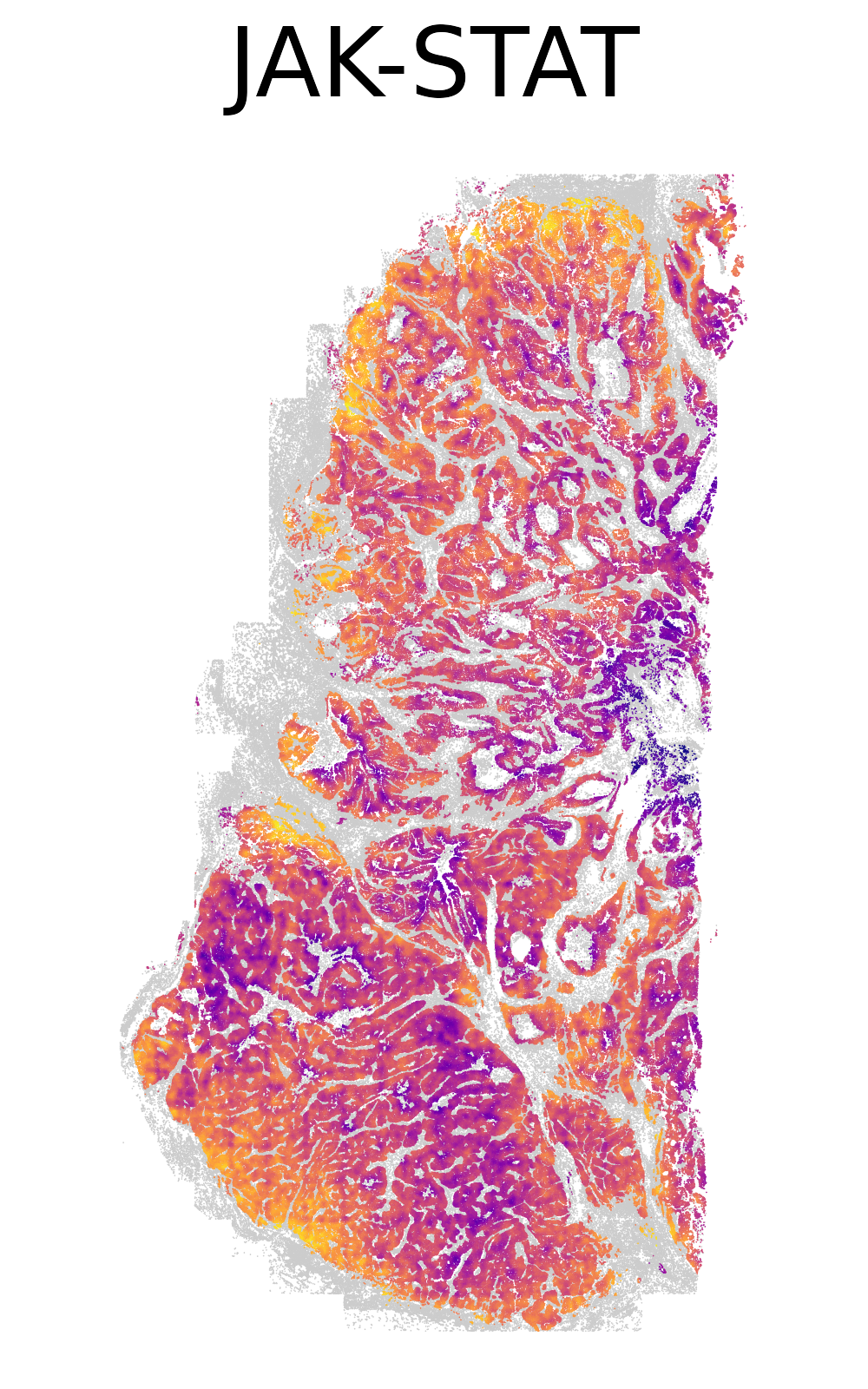
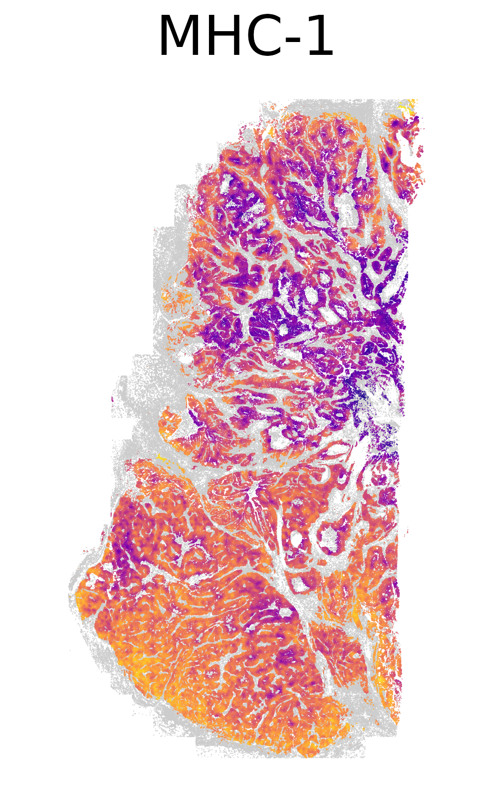
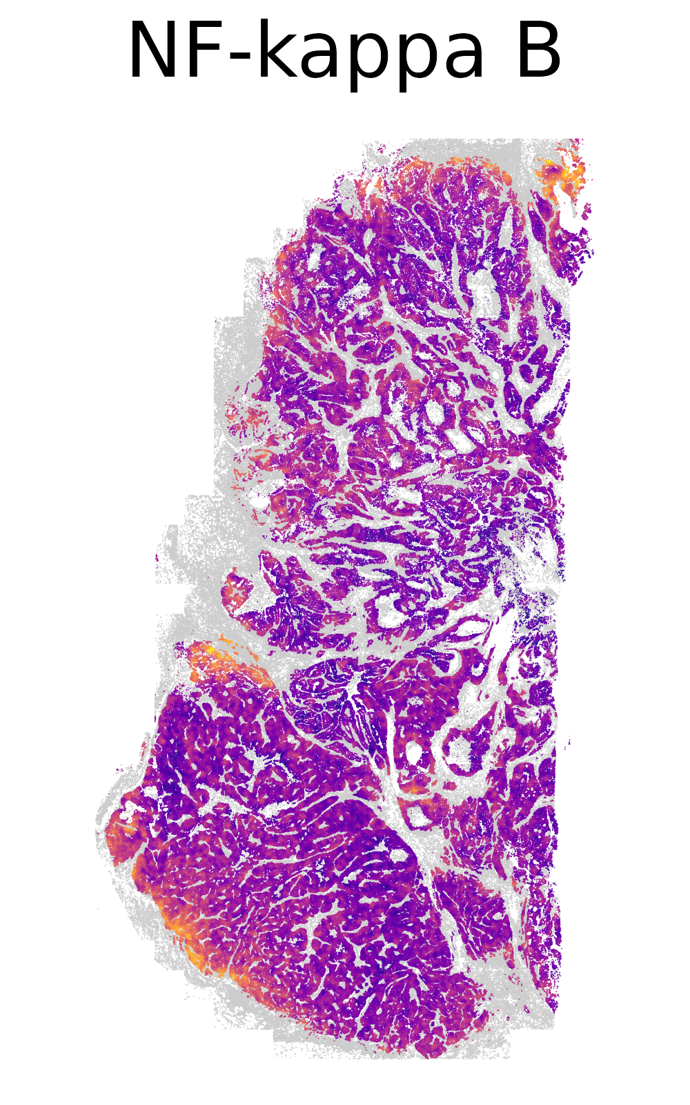
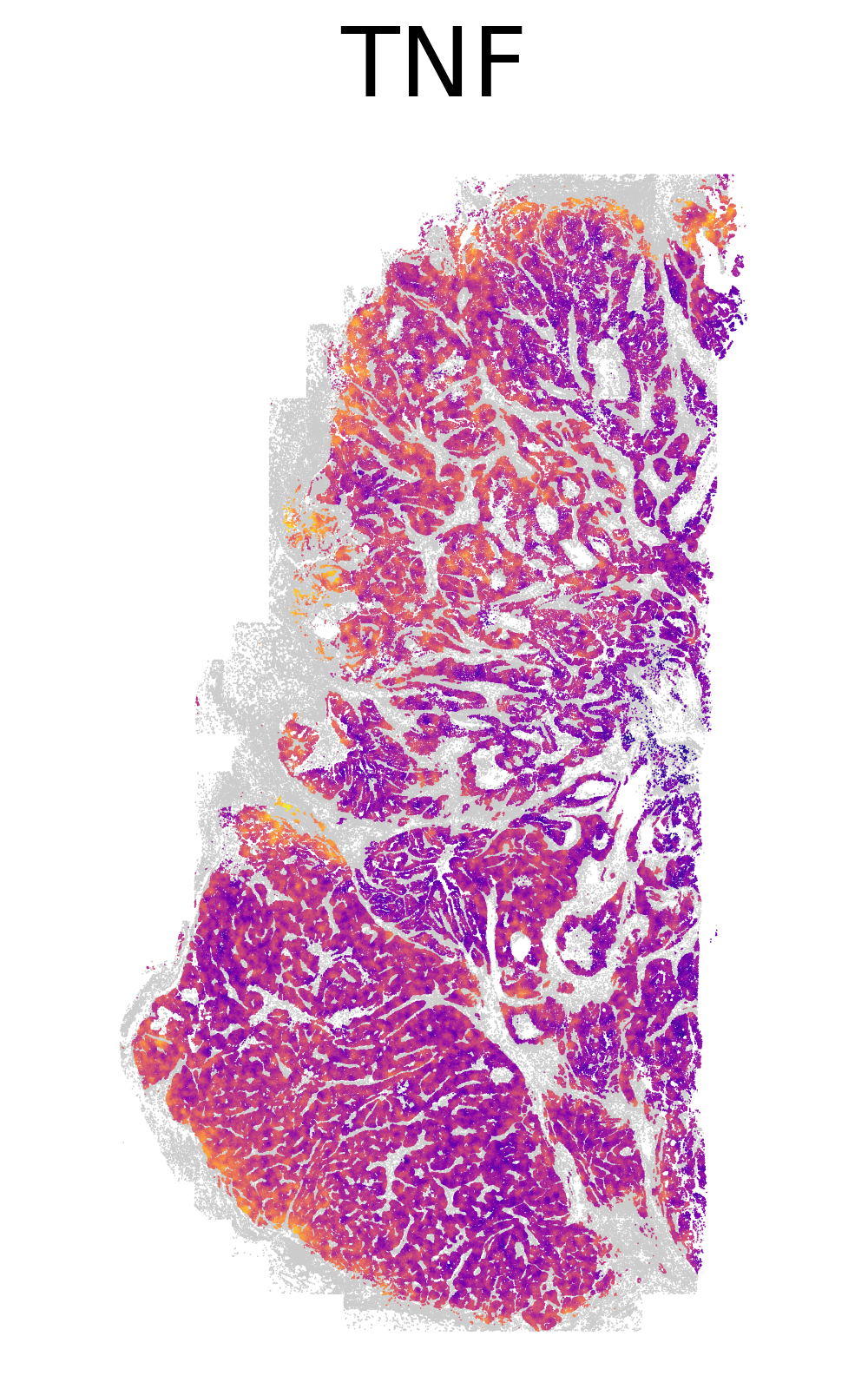
We generate spatial plots of a number of immune-related pathways, focusing only on expression within tumor cells. We perform spatial smoothing across tumor cells.
Show the code
# if there's no seurat object, read it inif (!("seu.obj"%in%ls())){ seu.obj <-readRDS(results_list$seurat_file_postCellTyping)}meta <- seu.obj@meta.data# Read in AUCell resultscells_auc_full <-readRDS(paste0(pathway_dir, "/Data/cellsAUC_" ,"full" ,".rds"))# Calculate smoothed neighborhood expressionxy <- seu.obj@meta.data[,c("x_slide_mm", "y_slide_mm")]xy$cell_ID <-rownames(xy)# Use a smoothing function modified from https://nanostring-biostats.github.io/CosMx-Analysis-Scratch-Space/posts/marker-gene-smoothing/xy_nn <-function(xy, n_neighbors=50){ xy <-as.data.table(xy)## identify nearest n_neighbors (+1 includes the cell as a neighbor to itself) nn_xy <- RANN::nn2(xy[,.(x_slide_mm, y_slide_mm)],k = n_neighbors +1)$nn.idx nn_xy <- data.table::melt(cbind(xy[,.(cell_ID)], data.table(nn_xy)) , id.vars=c("cell_ID", "V1"))colnames(nn_xy) <-c("cell_ID1", "cell_ID1_idx", "neighbor", "cell_ID2_idx") nn_xy <-merge(nn_xy , nn_xy[,.(cell_ID2=cell_ID1, cell_ID2_idx=cell_ID1_idx)][ ,unique(.SD)],by="cell_ID2_idx")## Cell x cell neighbor indicator matrix wxy <- Matrix::sparseMatrix(i =c(unique(nn_xy$cell_ID1_idx), nn_xy$cell_ID2_idx) ,j=c(unique(nn_xy$cell_ID1_idx), nn_xy$cell_ID1_idx) ,x=1)rownames(wxy) <-colnames(wxy) <- nn_xy[order(nn_xy$cell_ID1_idx),unique(cell_ID1)]## Column standardize, so that columns (cells) sum to 1, and each neighbor given equal weight. mxy <- Matrix::sparseMatrix(i=1:ncol(wxy) ,j=1:ncol(wxy) ,x=1/Matrix::colSums(wxy) )dimnames(mxy) <-dimnames(wxy) smoother <- mxy %*% wxy smoother <- smoother[,xy$cell_ID]return(smoother)}# Get smoother for tumor cells onlysmoother_tum <-xy_nn(xy[meta$major_cell_type =="Tumor",])# Plot four key pathways with abbreviated nameskey_pathways =c("JAK-STAT"="REACTOME_GENE_AND_PROTEIN_EXPRESSION_BY_JAK_STAT_SIGNALING_AFTER_INTERLEUKIN_12_STIMULATION","MHC-1"="REACTOME_ANTIGEN_PRESENTATION_FOLDING_ASSEMBLY_AND_PEPTIDE_LOADING_OF_CLASS_I_MHC","NF-kappa B"="REACTOME_REGULATION_OF_NF_KAPPA_B_SIGNALING","TNF"="REACTOME_TNF_SIGNALING")# Plot each pathwayfor(i in1:4){ pathway = key_pathways[i]# Extract pathway scorespath_score <- cells_auc_full[pathway,]meta$path_score <- path_score[meta$cell_ID]smoothed_path_score <- meta[which(meta$major_cell_type =="Tumor"),"path_score"] %*% smoother_tum# Save this smoothed pathway scoresaveRDS(smoothed_path_score, file =paste0(immNeigh_dir, "/Data/xy_smoothed_tumor_", pathway, ".rds"))# Plot smoothed pathway in spacemeta$smoothed_path_score <-NAmeta[which(meta$major_cell_type =="Tumor"), "smoothed_path_score"] <- smoothed_path_score[1,]ggplot(meta %>%filter(major_cell_type !="Tumor"), aes(x = x_slide_mm, y = y_slide_mm)) +geom_point(size =0.01, color ="grey80", stroke =0.1) +geom_point(data = meta %>%filter(major_cell_type =="Tumor"),aes(x_slide_mm, y_slide_mm, color = smoothed_path_score),size =0.01, stroke =0.1) +scale_color_viridis(option ="plasma") +coord_fixed() +theme_void() +ggtitle(paste0(names(key_pathways)[i])) +theme(legend.position ="none", plot.title =element_text(hjust =0.5, size =20))ggsave(filename =paste0(immNeigh_dir, "/Plots/XY_smoothed_tumor_", gsub("-", "_", names(key_pathways)[i]), ".png"),width =2.5, height =4, units ="in", dpi =400)}
Spatial plots of the smoothed immune-related pathways in tumor cells.
We group CD8 T cytotoxic cells by novae-defined niches and ask how their transcriptomes differ between broad neighborhoods. We predict that as T cells move more deeply into the tumor, they will become activated or they will go past this to an exhausted state.
5.3.1 Definition of three niches
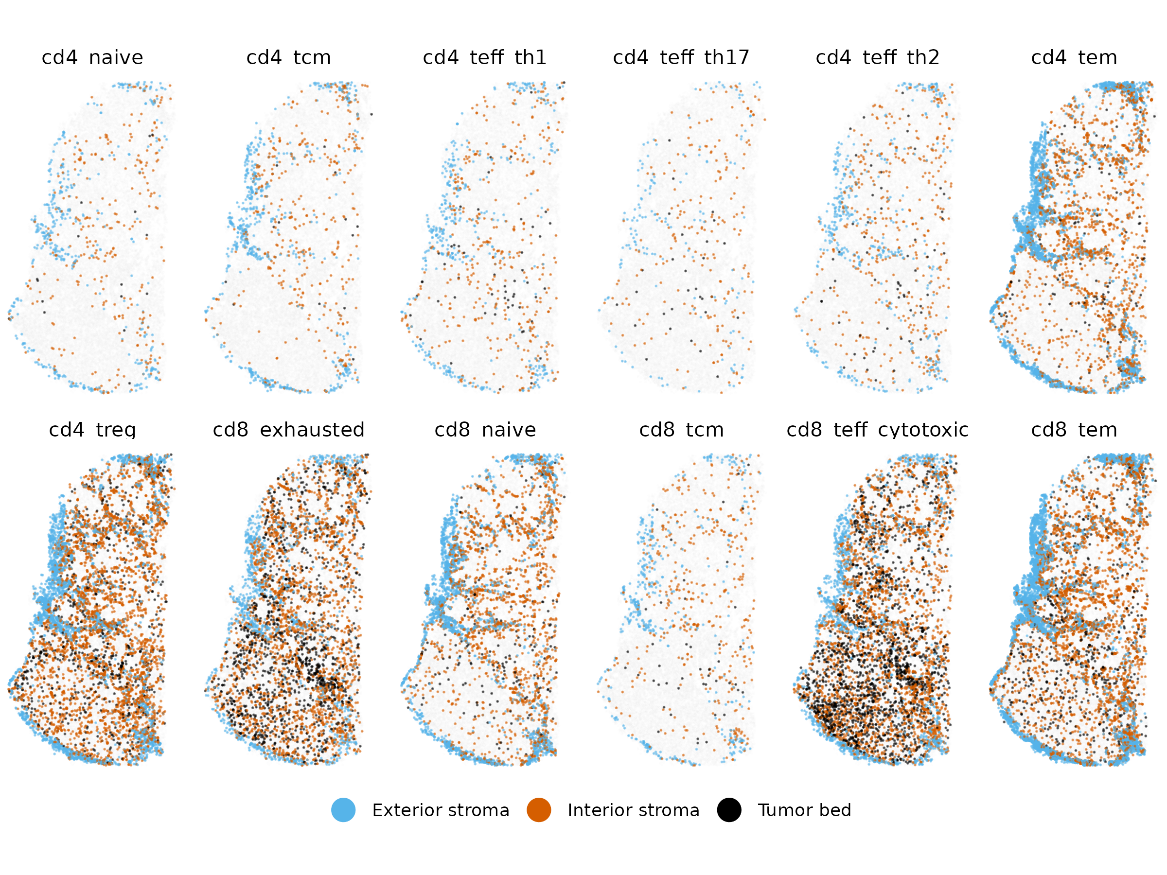
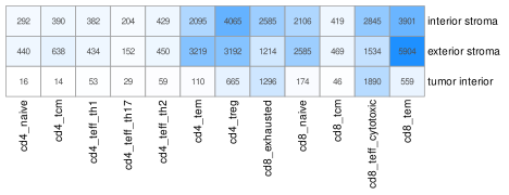
Generate a gallery of T cell subtypes showing their distribution across three niches
Show the code
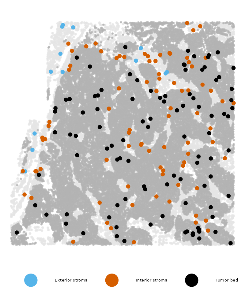
if(!("seu.obj"%in%ls())){ seu.obj <-readRDS(results_list$seurat_file_postCellTyping)}# Read in novae domain assignmentsnovae_9 <-readRDS(file =paste0(niche_dir, "/Data/novae_domains_9_assignments.rds"))# Add to metadatameta <- seu.obj@meta.datameta$novae_9 <- novae_9[row.names(meta)]# Add broad niche assignmentsexteriornames <-paste0("D", c(987, 1003))interiornames <-paste0("D", c(1014,1007,1008, 1011))tumornames <-paste0("D", c(1012,1013,976))bigniche <-as.character(novae_9)bigniche[is.element(novae_9, exteriornames)] <-"Exterior stroma"bigniche[is.element(novae_9, interiornames)] <-"Interior stroma"bigniche[is.element(novae_9, tumornames)] <-"Tumor bed"names(bigniche) <-names(novae_9)meta$broad_niche_v2 <- bigniche[row.names(meta)]# For this plot, remove any cells which are not assigned a niche (this is 16 cells)meta <- meta[!is.na(meta$broad_niche_v2),]# Plot only T cellsidx =which(meta$major_cell_type %in%c("Tcell"))ggplot(meta[idx,],aes(x = x_slide_mm, y = y_slide_mm)) +geom_point(data = df2, color ="grey90", size =0.01, alpha =0.05) +# Background cellsgeom_point(aes(color = broad_niche_v2), size =0.01, alpha =0.5)+# Foreground highlighted cellsscale_color_manual(values =c("Exterior stroma"="#56B4E9","Interior stroma"="#D55E00","Tumor bed"="#000000"), name ="") +coord_fixed() +theme_void() +facet_wrap(~minor_cell_type, nrow =2) +theme(strip.text =element_text(size =10)) +guides(color =guide_legend(override.aes =list(size =5, alpha =1))) +theme(legend.direction ="horizontal", # Arrange items within a legend horizontallylegend.position ="bottom"# Place the entire legend box at the bottom )ggsave(paste0(immNeigh_dir, "/Plots/gallery_TCells_broadNiche2.png"),width =8, height =6, units ="in")# Make a zoomed in plot of CD8 cytotoxic showing three colors plus tumoridx =which(meta$minor_cell_type =="cd8_teff_cytotoxic")ggplot(meta[idx,],aes(x = x_slide_mm, y = y_slide_mm)) +geom_point(data = meta %>%filter(major_cell_type !="Tumor"), color ="grey90", size =0.1, alpha =0.7) +# Background cellsgeom_point(data = meta %>%filter(major_cell_type =="Tumor"), color ="grey70", size =0.01, alpha =0.7) +# Tumor cellsgeom_point(aes(color = broad_niche_v2), size =0.5, alpha =1)+# Foreground highlighted cellsscale_color_manual(values =c("Exterior stroma"="#56B4E9","Interior stroma"="#D55E00","Tumor bed"="#000000"), name ="") +coord_fixed() +theme_void() +guides(color =guide_legend(override.aes =list(size =3, alpha =1))) +theme(legend.direction ="horizontal", # Arrange items within a legend horizontallylegend.position ="bottom", # Place the entire legend box at the bottomlegend.text =element_text(size =2.5) ) +xlim(c(0.7, 2.7)) +ylim(c(4,6))ggsave(paste0(immNeigh_dir, "/Plots/XY_TCD8cytotoxic_broadNiche2_zoom.png"),width =2, height =2.5, units ="in", dpi =400)
Gallery of spatial plots of all T cell subtypes, colored by broad niche:
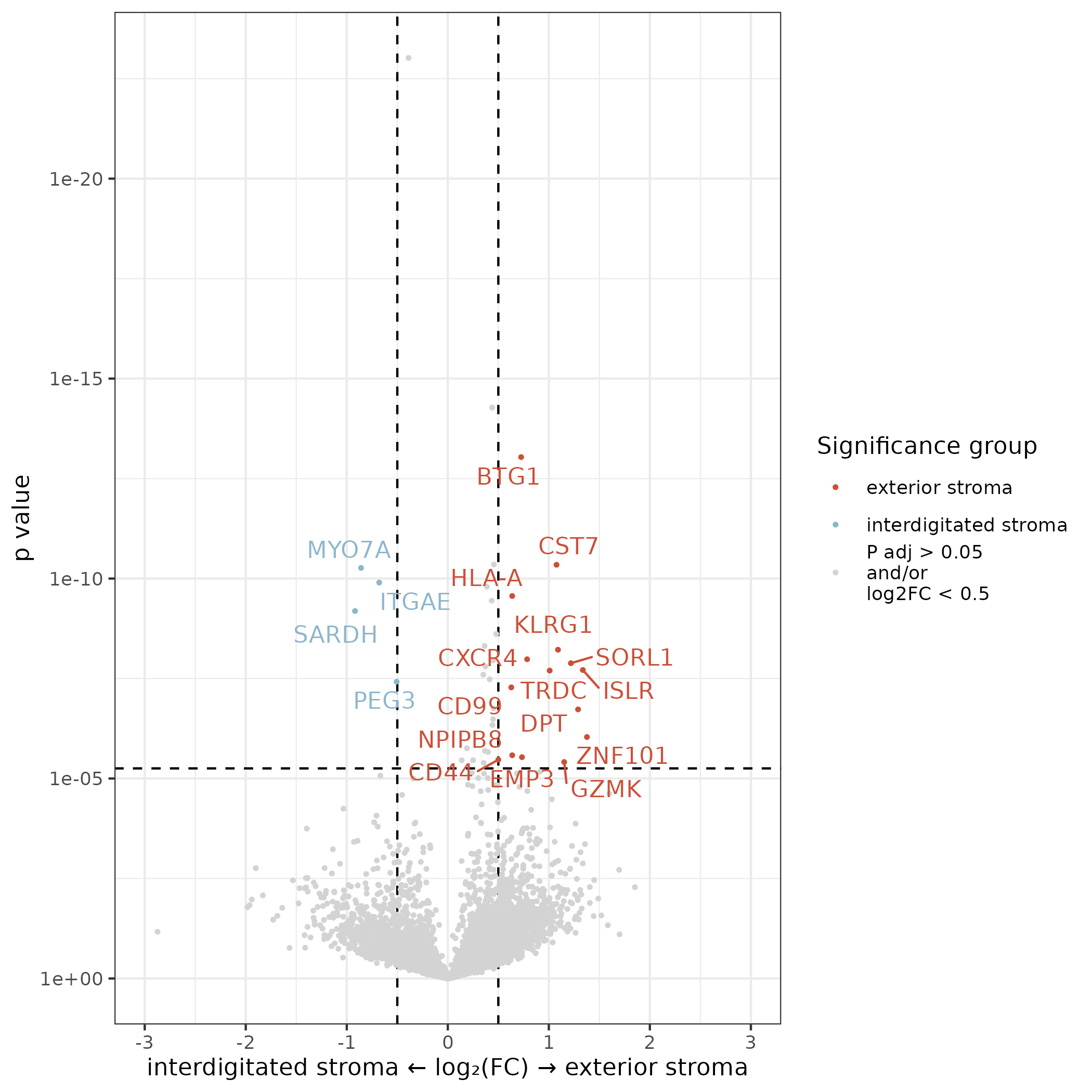
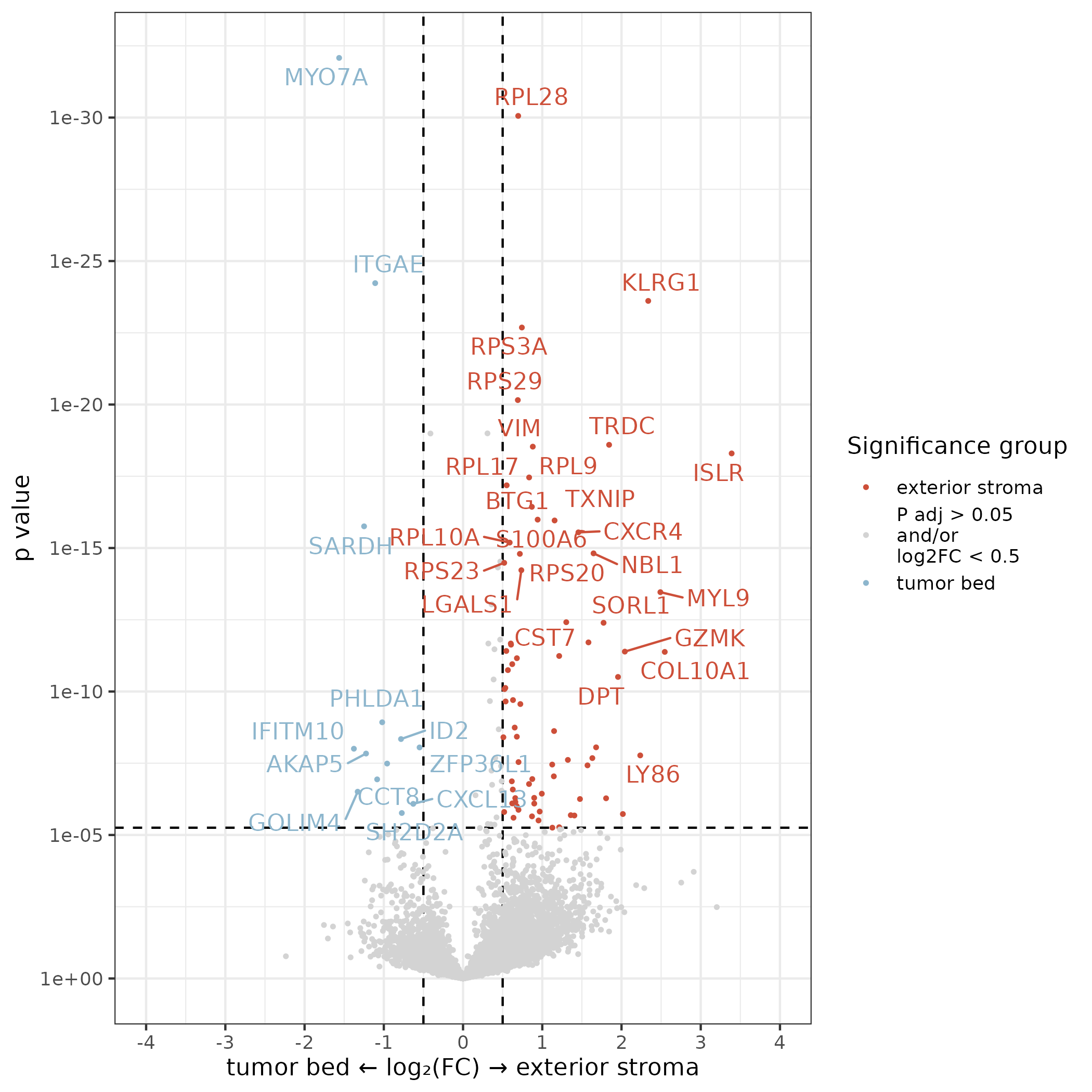
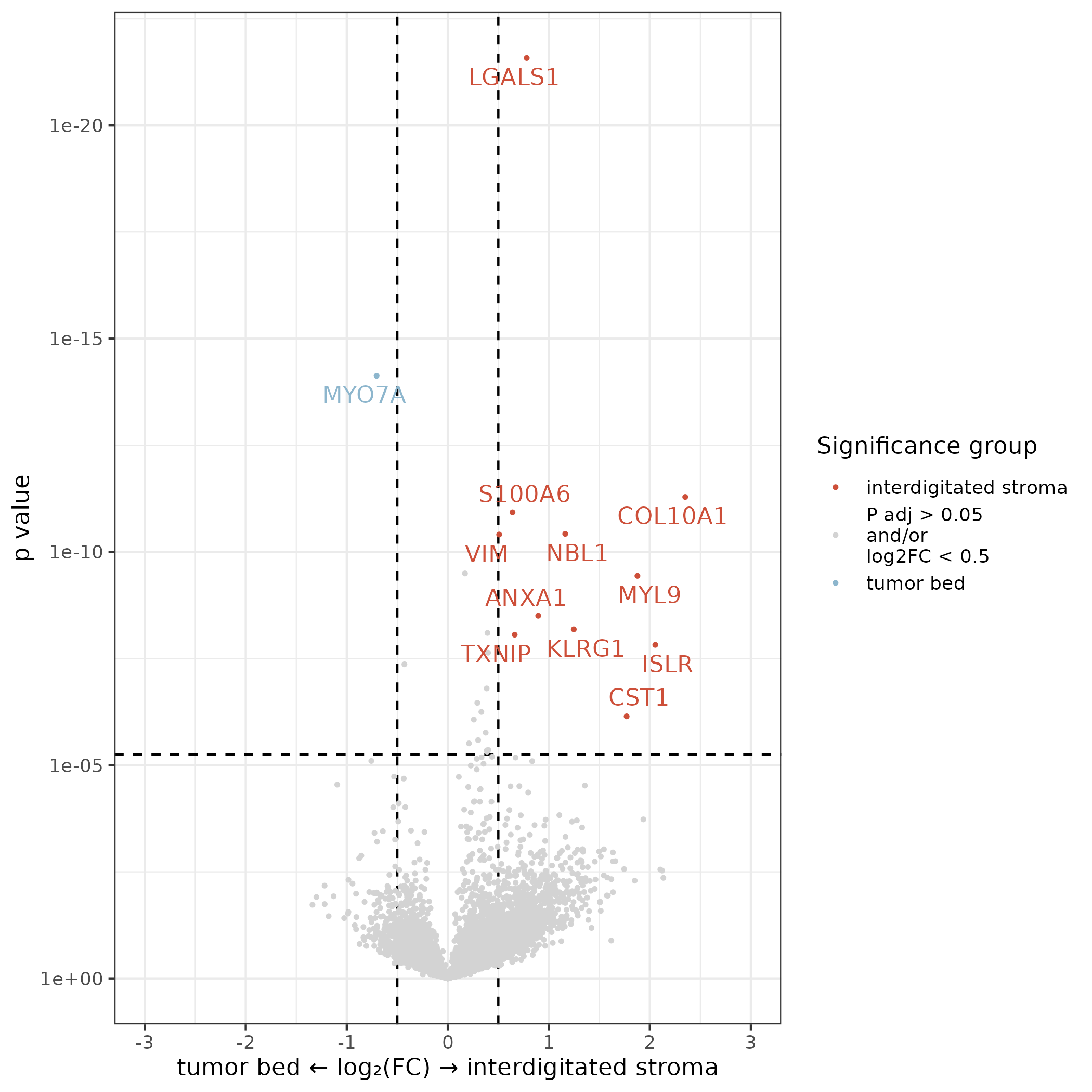
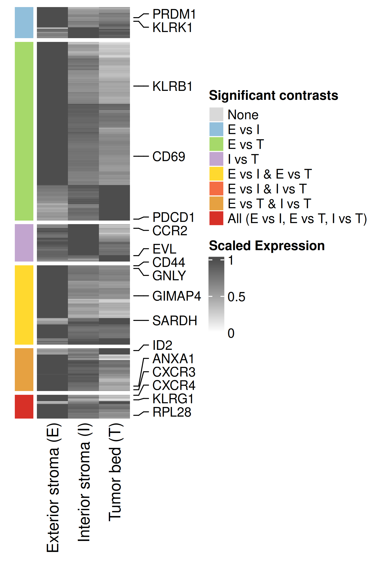
In addition to these volcano plots for each pairwise comparison, we make one summary plot that shows estimated mean for each broad niche and pairwise significance. Estimated mean is shown relative to the location with the highest expression. Only genes reaching significance in at least one pairwise comparison are shown. Also save the table of DE results to be provided as a supplementary table.
Show the code
# Read in DE objectde_obj <-readRDS(paste0(immNeigh_dir, "/Data/cd8teff_broadNiche_de_obj.rds"))# Extract estimated meansem_res <-results(de_obj)$emmeans %>%filter(term =="broad_niche")# Extract pairwise resultspairwise.df <-results(de_obj, "pairwise")$pairwise# Conversions of some data namesif("broad_niche_v2"%in% pairwise.df$term){ pairwise.df$term =gsub("broad_niche_v2", "broad_niche", pairwise.df$term)}pairwise.df <- pairwise.df %>%filter(term =="broad_niche")# Add fdrpairwise.df$fdr =p.adjust(pairwise.df$p.value, method ="fdr")# Save pairwise results to a table to be included as supplementary information.write.csv(as.data.frame(pairwise.df)[,c(setdiff(colnames(pairwise.df), c("df", "null", "fold_change")))],file =paste0(immNeigh_dir, "/Data/CD8TcytotoxicBroadNicheDE_table.csv"),row.names =FALSE)# Select all genes that have fdr < 0.05 in any comparisonde_genes <- pairwise.df %>%filter(fdr <0.05) %>%pull(target) %>%unique()# Extract estimated means for all de genesem_de <- em_res %>%filter(target %in% de_genes)# Filter for significant genes (FDR < 0.05) and count number and type of DE comparisons per genede_signature <- pairwise.df %>%filter(fdr <0.05) %>%distinct(target, contrast) %>%group_by(target) %>%summarise(de_signature =paste(sort(unique(contrast)), collapse ="_"),.groups ="drop" )# Prepare expression matrixexpr_matrix <- em_de %>% dplyr::select(target, level, response) %>%pivot_wider(names_from = level, values_from = response) %>%column_to_rownames("target")# Scale each row to [0, 1] by dividing by row maxexpr_scaled <-t(apply(expr_matrix, 1, function(x) x /max(x, na.rm =TRUE)))# Create annotation for DE count# Merge DE count with expression matrix rownamesde_annotation <-data.frame(target =rownames(expr_scaled)) %>%left_join(de_signature, by ="target") # Define color palette for DE signaturede_levels <-c("none", # no DE"exterior stroma / interior stroma","exterior stroma / tumor bed","interior stroma / tumor bed","exterior stroma / interior stroma_exterior stroma / tumor bed","exterior stroma / interior stroma_interdigitated stroma / tumor bed","exterior stroma / tumor bed_interior stroma / tumor bed","exterior stroma / interior stroma_exterior stroma / tumor bed_interior stroma / tumor bed")de_annotation$de_signature <-factor(de_annotation$de_signature,levels = de_levels)# Assign colors based on number of comparisonsde_colors <-c("none"="#d9d9d9", # neutral gray"exterior stroma / interior stroma"="#91bfdb", # cool blue"exterior stroma / tumor bed"="#a6d96a", # cool green"interior stroma / tumor bed"="#c2a5cf", # cool purple"exterior stroma / interior stroma_exterior stroma / tumor bed"="#ffd92f", # bright yellow"exterior stroma / interior stroma_interior stroma / tumor bed"="#f46d43", # warm coral"exterior stroma / tumor bed_interior stroma / tumor bed"="#e6a141", # warm amber"exterior stroma / interior stroma_exterior stroma / tumor bed_interior stroma / tumor bed"="#d73027"# hot red)## Cluster genes within each group# Create a list to store ordered gene namesordered_genes <-c()# Loop through each DE signature groupfor (group in de_levels) { genes_in_group <- de_annotation %>%filter(de_signature == group) %>%pull(target)if (length(genes_in_group) >1) {# Subset expression matrix submatrix <- expr_scaled[genes_in_group, ]# Compute hierarchical clustering hc <-hclust(dist(submatrix))# Get ordered gene names ordered_genes <-c(ordered_genes, genes_in_group[hc$order]) } else {# If only one gene, just add it ordered_genes <-c(ordered_genes, genes_in_group) }}# Set gene order for expression matrix and annotationexpr_scaled_ordered <- expr_scaled[ordered_genes, ]# Reorder annotation to matchde_annotation_ordered <- de_annotation[match(ordered_genes, de_annotation$target), ]# Use shorter DE signature names# Mapping long DE signature strings to short labelsde_signature_labels <-c("none"="None","exterior stroma / interior stroma"="E vs I","exterior stroma / tumor bed"="E vs T","interior stroma / tumor bed"="I vs T","exterior stroma / interior stroma_exterior stroma / tumor bed"="E vs I & E vs T","exterior stroma / interior stroma_interior stroma / tumor bed"="E vs I & I vs T","exterior stroma / tumor bed_interior stroma / tumor bed"="E vs T & I vs T","exterior stroma / interior stroma_exterior stroma / tumor bed_interior stroma / tumor bed"="All (E vs I, E vs T, I vs T)")names(de_colors) <- de_signature_labels[names(de_colors)]# Apply to factor levelsde_annotation_ordered$de_signature <-factor( de_annotation_ordered$de_signature,levels =names(de_signature_labels),labels = de_signature_labels)# Create row annotationrow_ha <-rowAnnotation(DE_Signature = de_annotation_ordered$de_signature,col =list(DE_Signature = de_colors),show_annotation_name =FALSE,annotation_legend_param =list(DE_Signature =list(title ="Significant contrasts") ))## Label specific genes of interest# Identify two representative genes per group# Add gene names to expression matrixexpr_scaled_ordered_df <-as.data.frame(expr_scaled_ordered)expr_scaled_ordered_df$target <-rownames(expr_scaled_ordered_df)# Target list chosen based on expected biology, unexpected but plausible, and present in one or more contrastsgenes_of_interest <-c("PDCD1", "KLRG1", "CXCR4", "RPL28", "SARDH", "CD69","KLRB1", "GIMAP4", "CD44","PRDM1", "KLRK1", "CCR2", "EVL", "GNLY", "H2BC4", "H1-4", "ID2", "CXCR3", "ANXA1")# Find the indices of these genes in the matrixgene_indices =which(rownames(expr_scaled_ordered) %in% genes_of_interest)# Create a row annotation with anno_mark()# This annotation will place the gene labels on the right side.gene_labels_anno =rowAnnotation(gene_labels =anno_mark(at = gene_indices,labels =rownames(expr_scaled_ordered)[gene_indices],labels_gp =gpar(fontsize =10), # Adjust label font sizelink_width =unit(5, "mm") # Adjust line length ))# Rename columns to include shorthandcolnames(expr_scaled_ordered) <- dplyr::recode(colnames(expr_scaled_ordered),"exterior stroma"="Exterior stroma (E)","interior stroma"="Interior stroma (I)","tumor bed"="Tumor bed (T)")# Generate heatmaphm <-Heatmap( expr_scaled_ordered,name ="Scaled Expression",col =colorRamp2(c(0, 1), c("white", "grey30")),cluster_rows =FALSE,cluster_columns =TRUE,show_row_names =FALSE,left_annotation = row_ha,row_split = de_annotation_ordered$de_signature,row_title_gp =gpar(fontsize =0),show_row_dend =FALSE,show_column_dend =FALSE,right_annotation = gene_labels_anno)png(filename =paste0(immNeigh_dir, "/Plots/heatmap_cd8teff_broadNiche_v2_selectedGenes.png"),width =4, height =6, units ="in", res =400)draw(hm)dev.off()
Heatmap of genes differentially expressed across broad niches: