3  Spatial domains

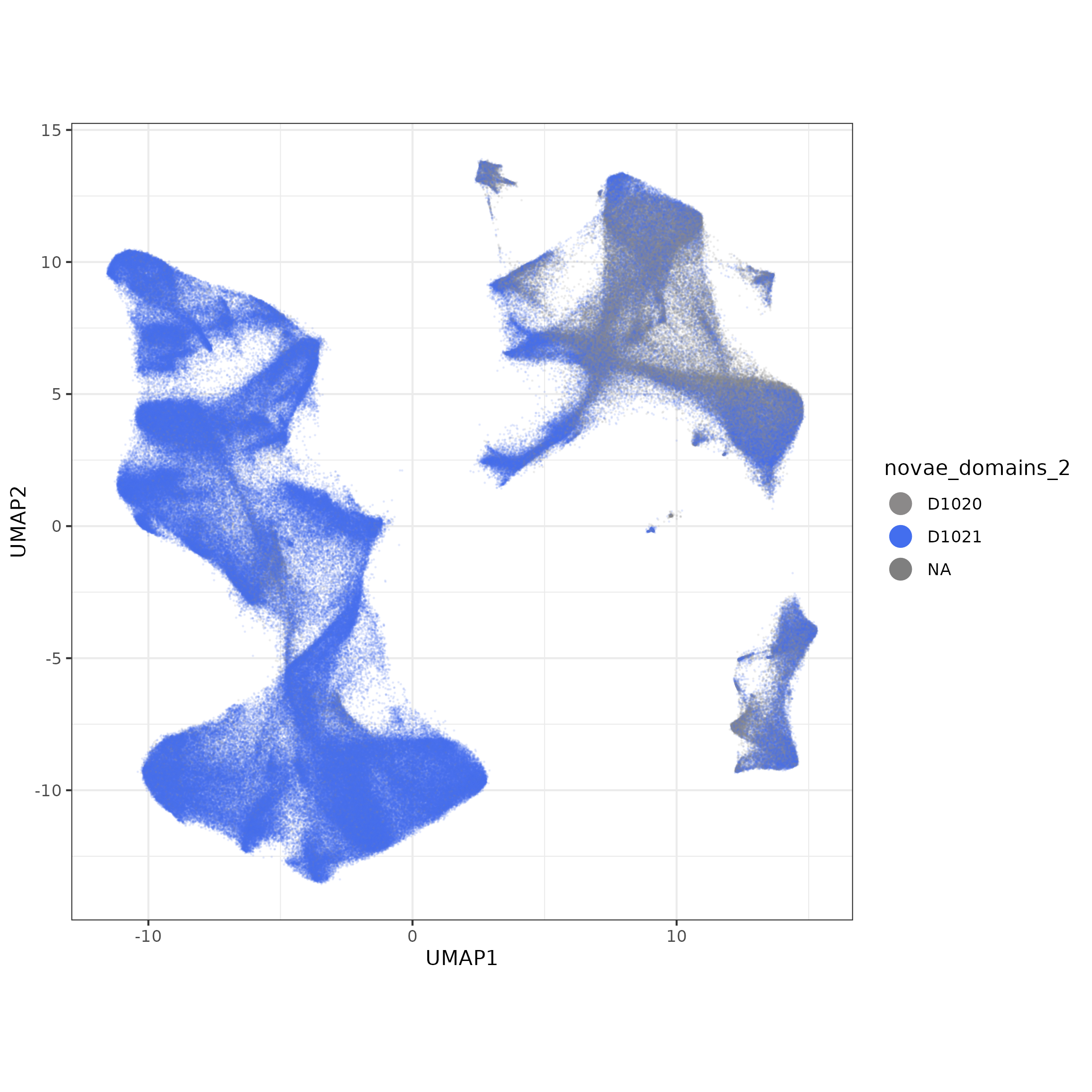
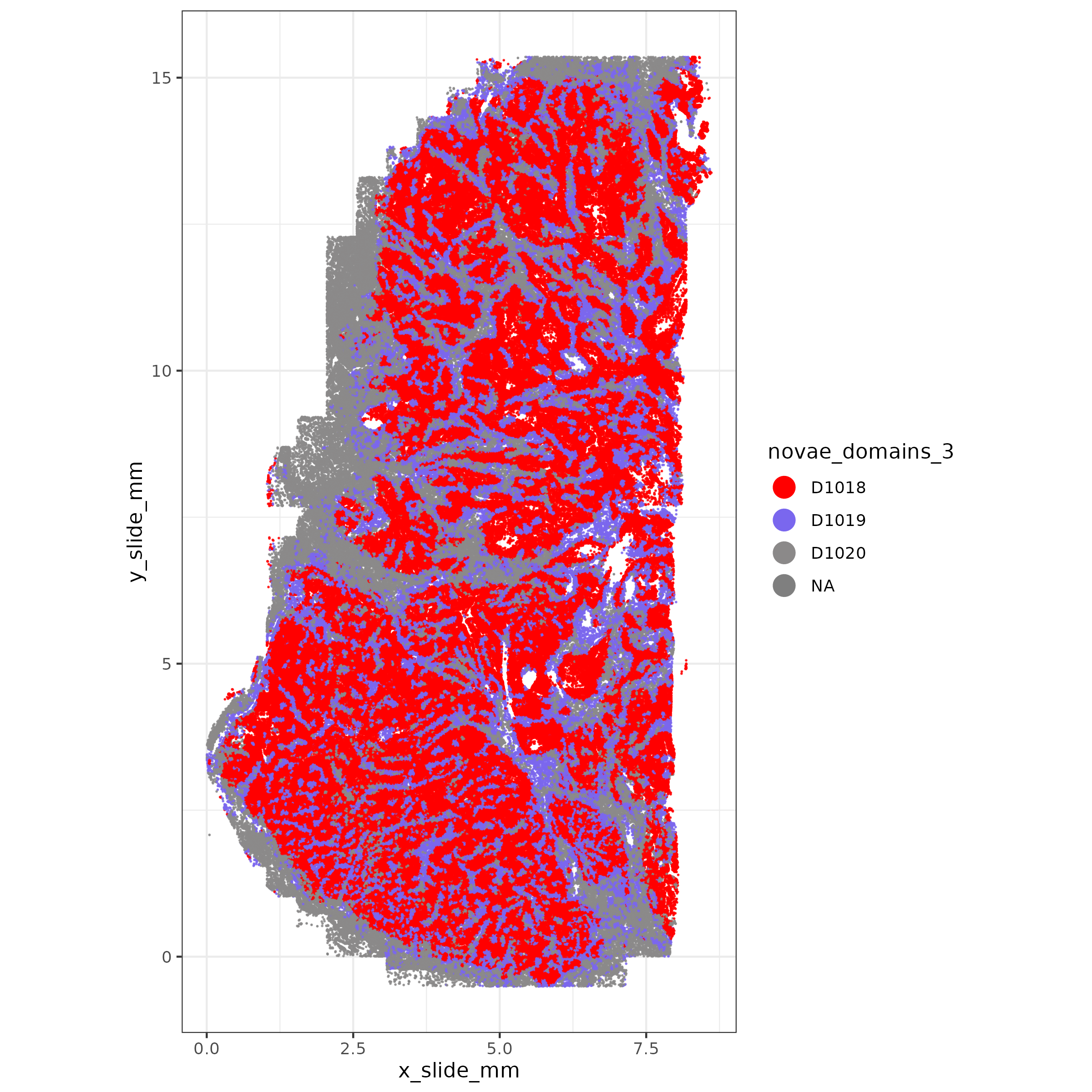
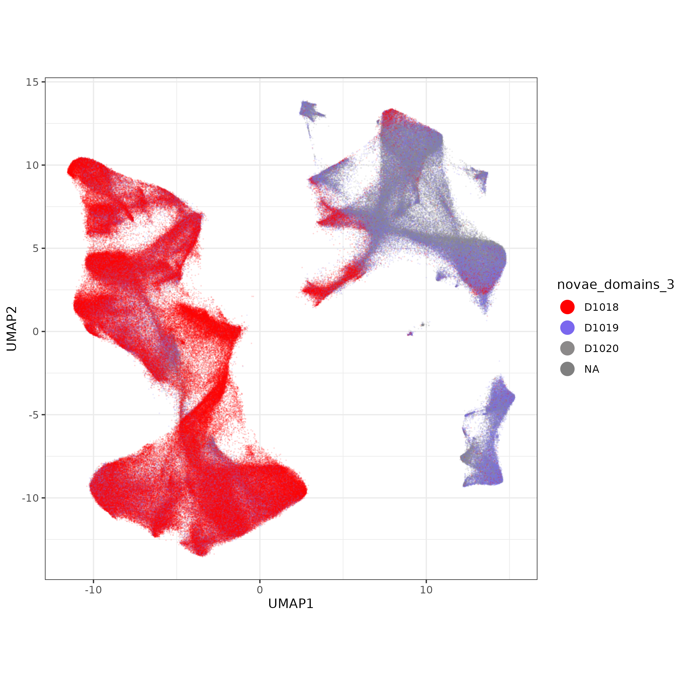
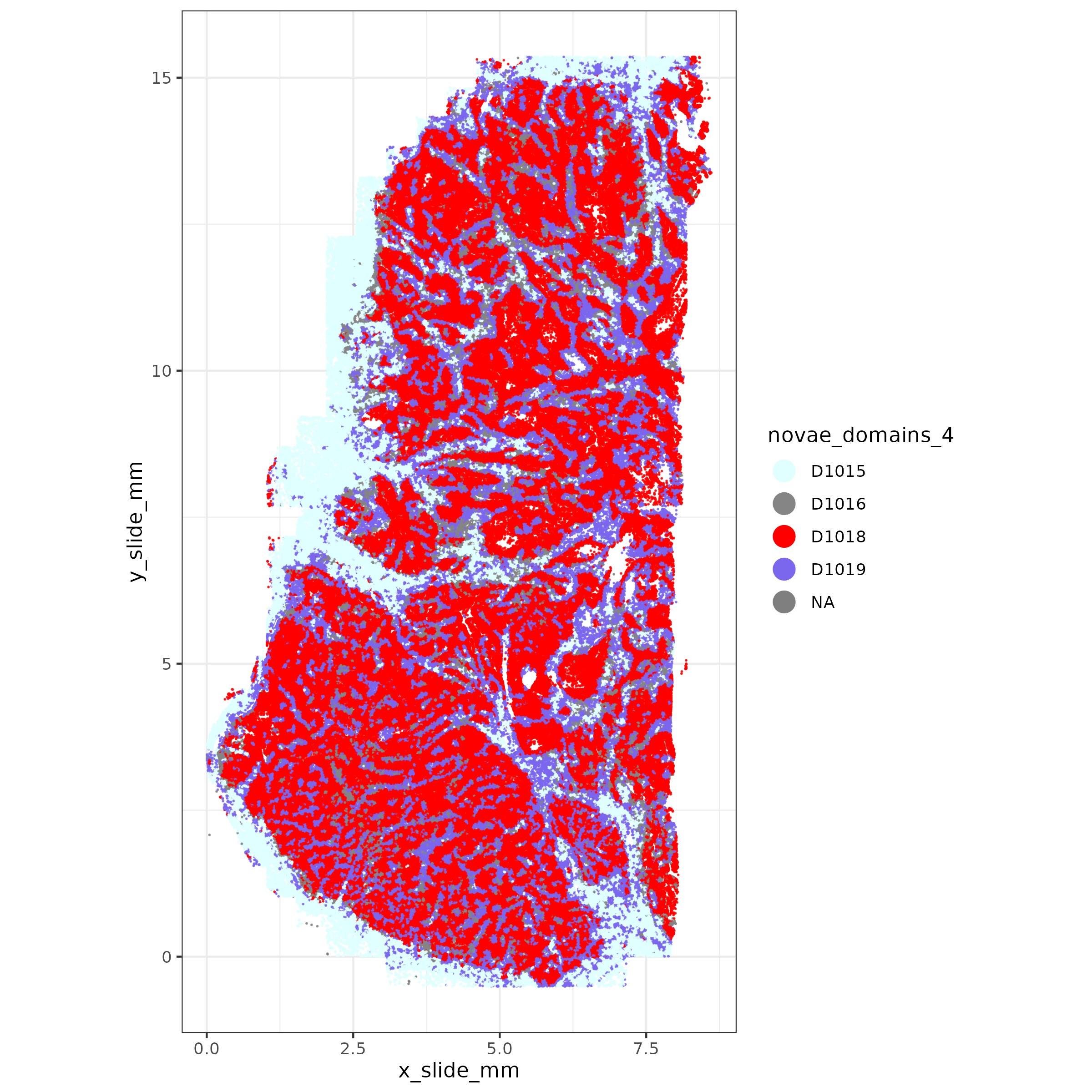
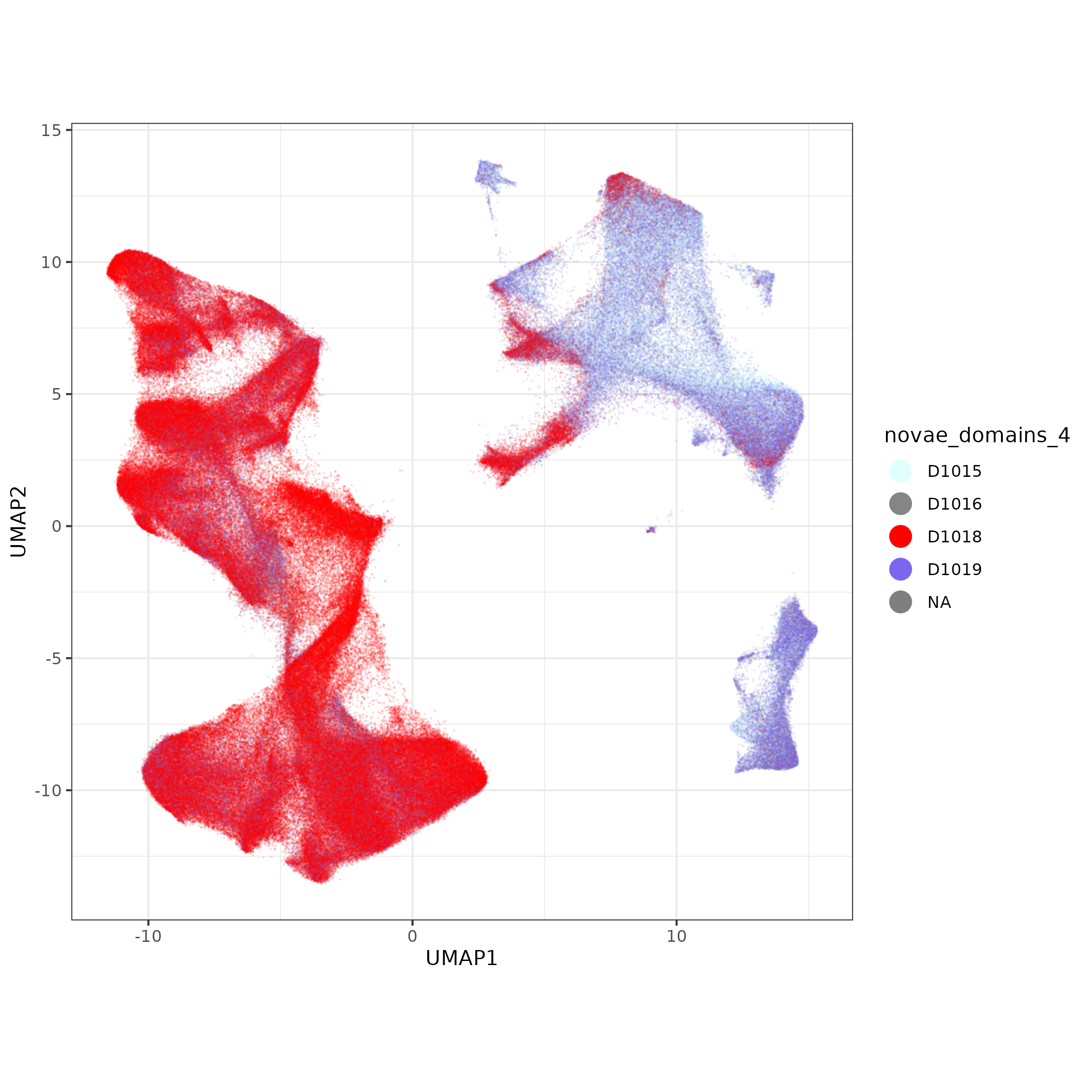
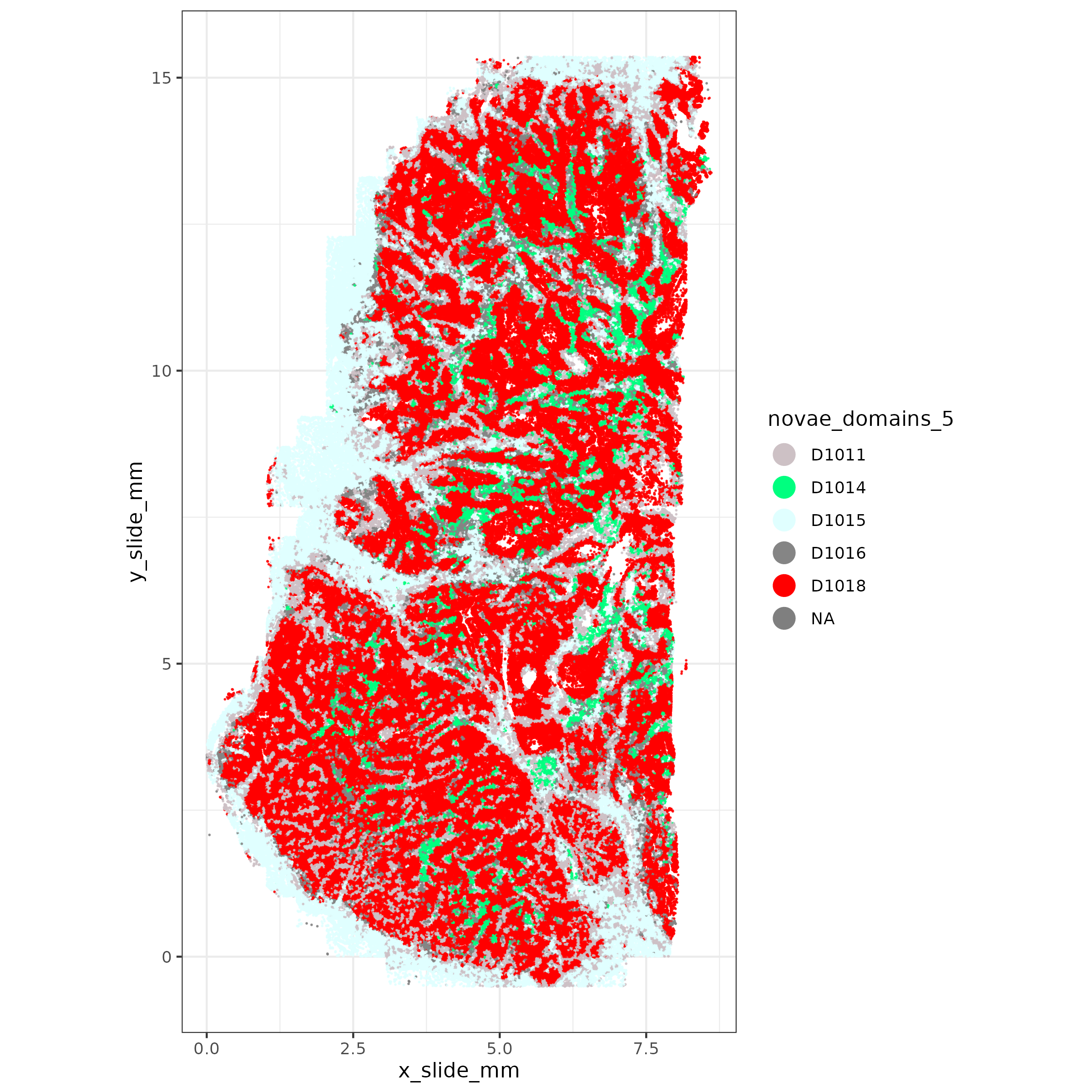
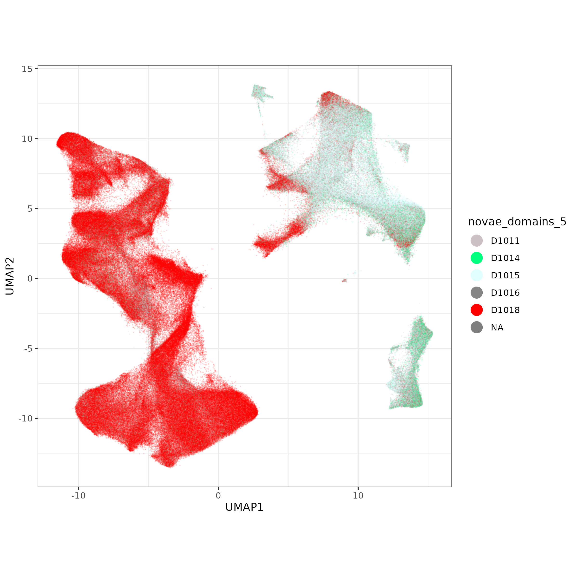
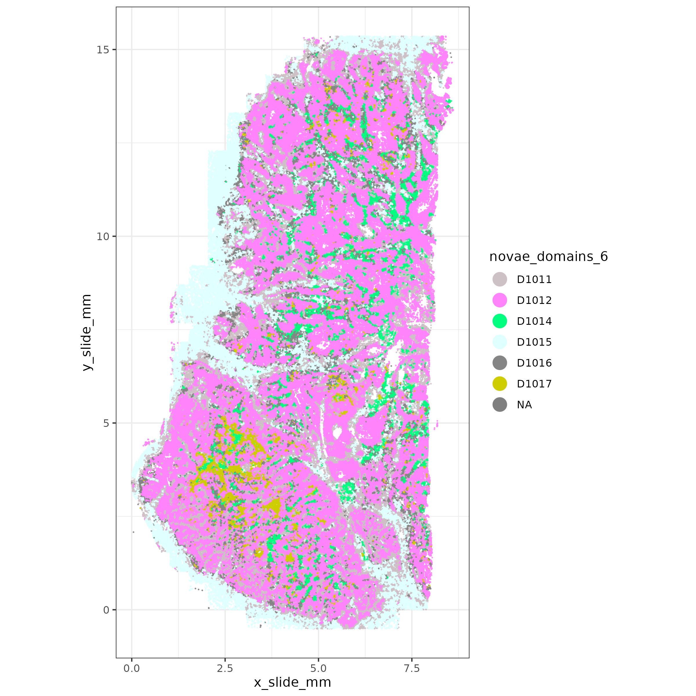
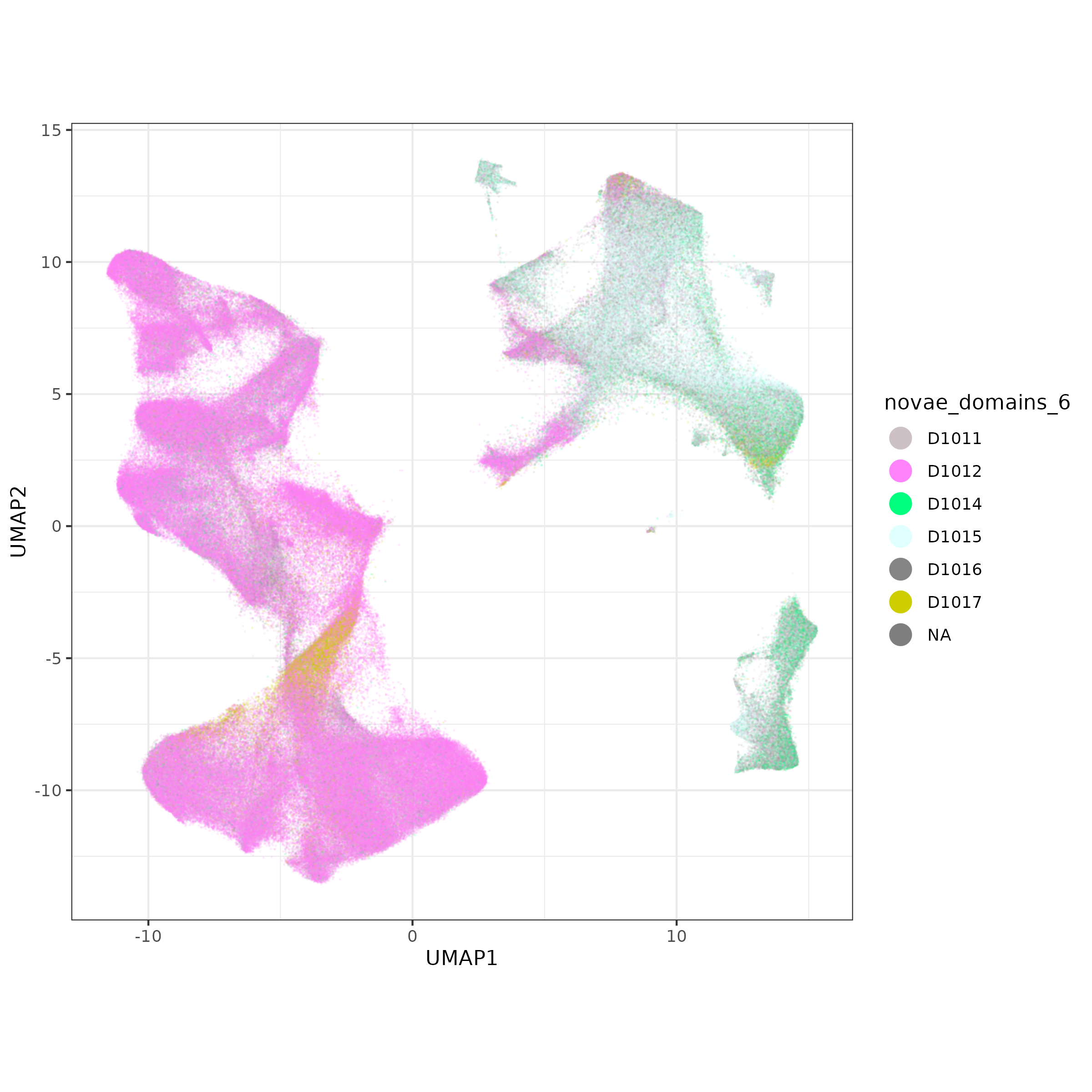
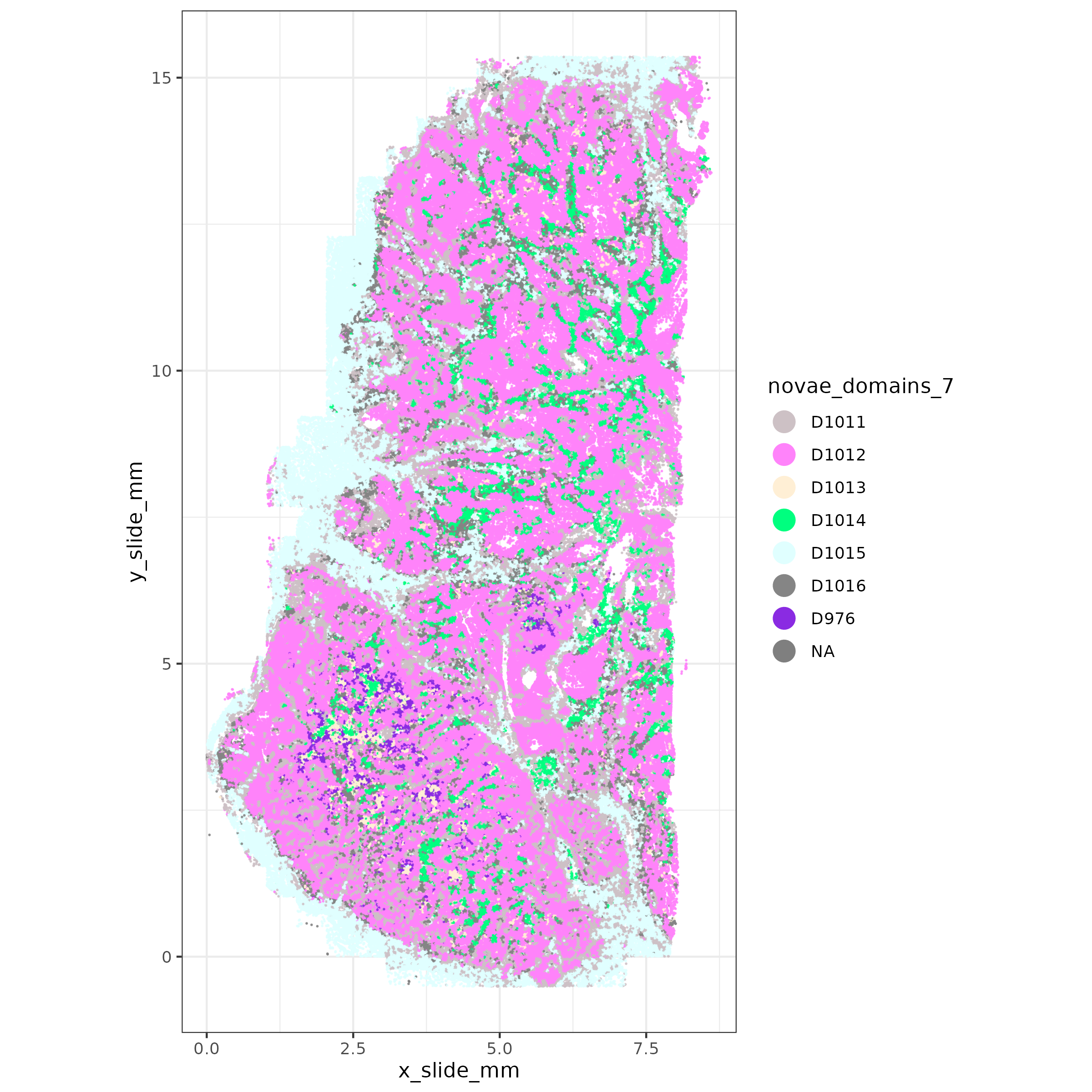
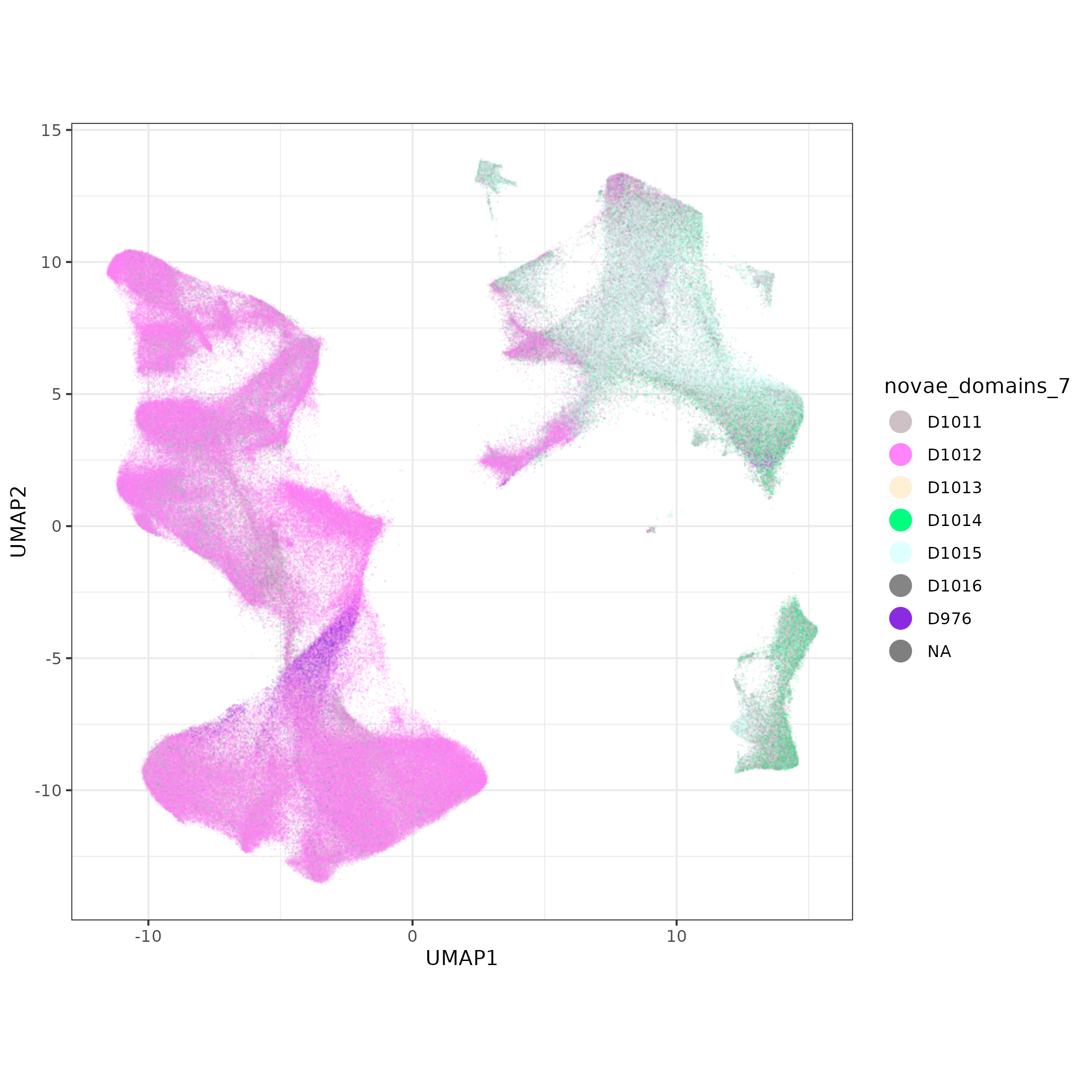
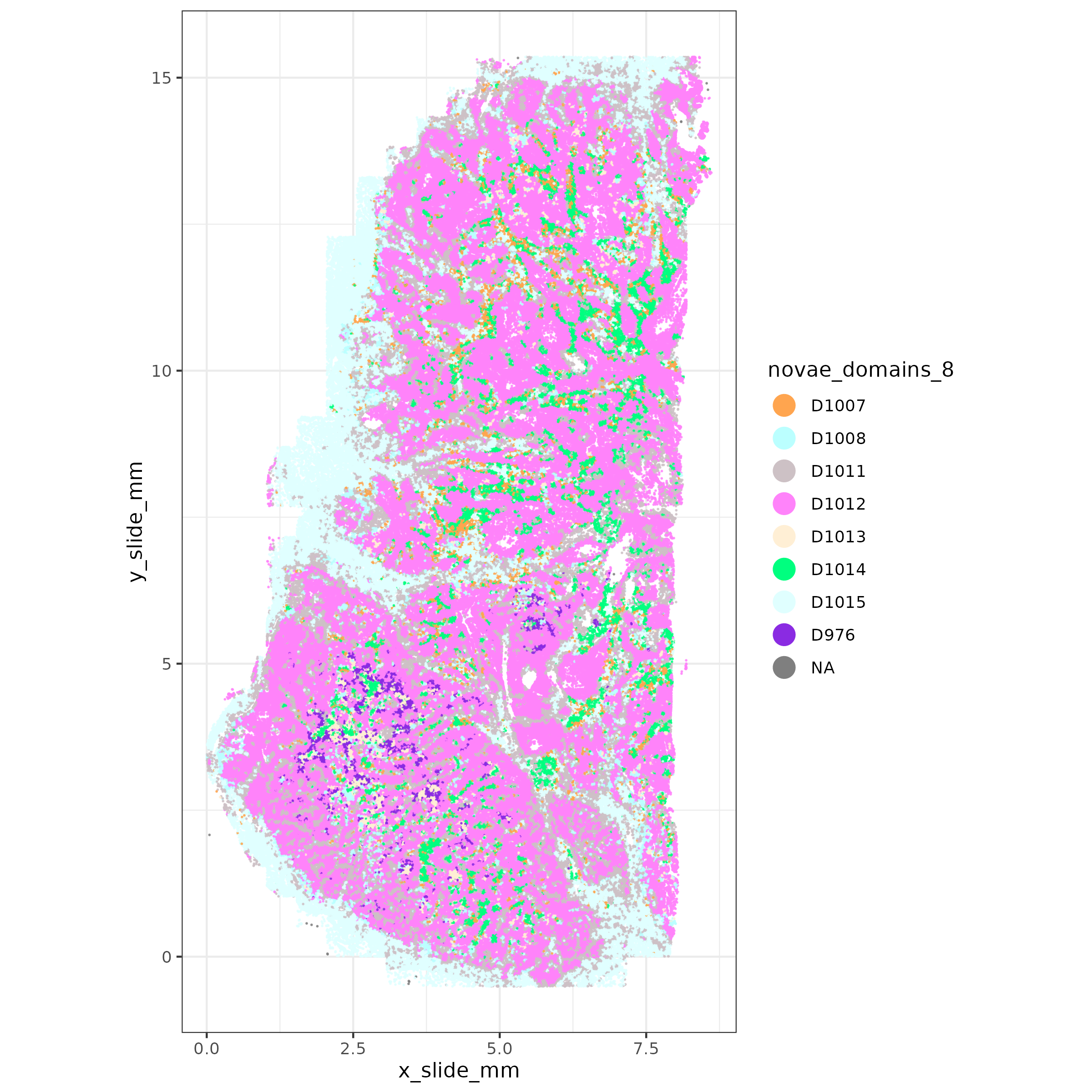
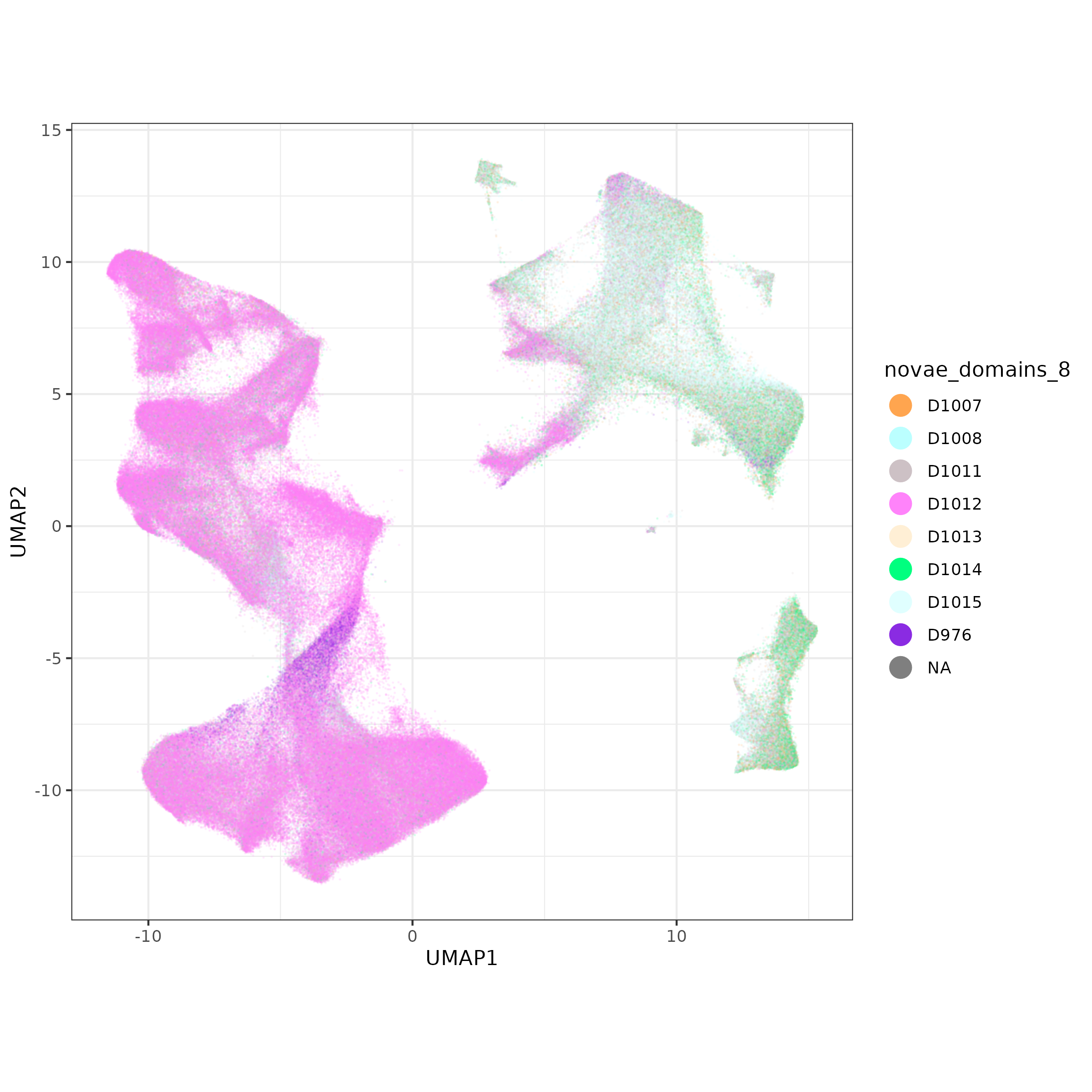
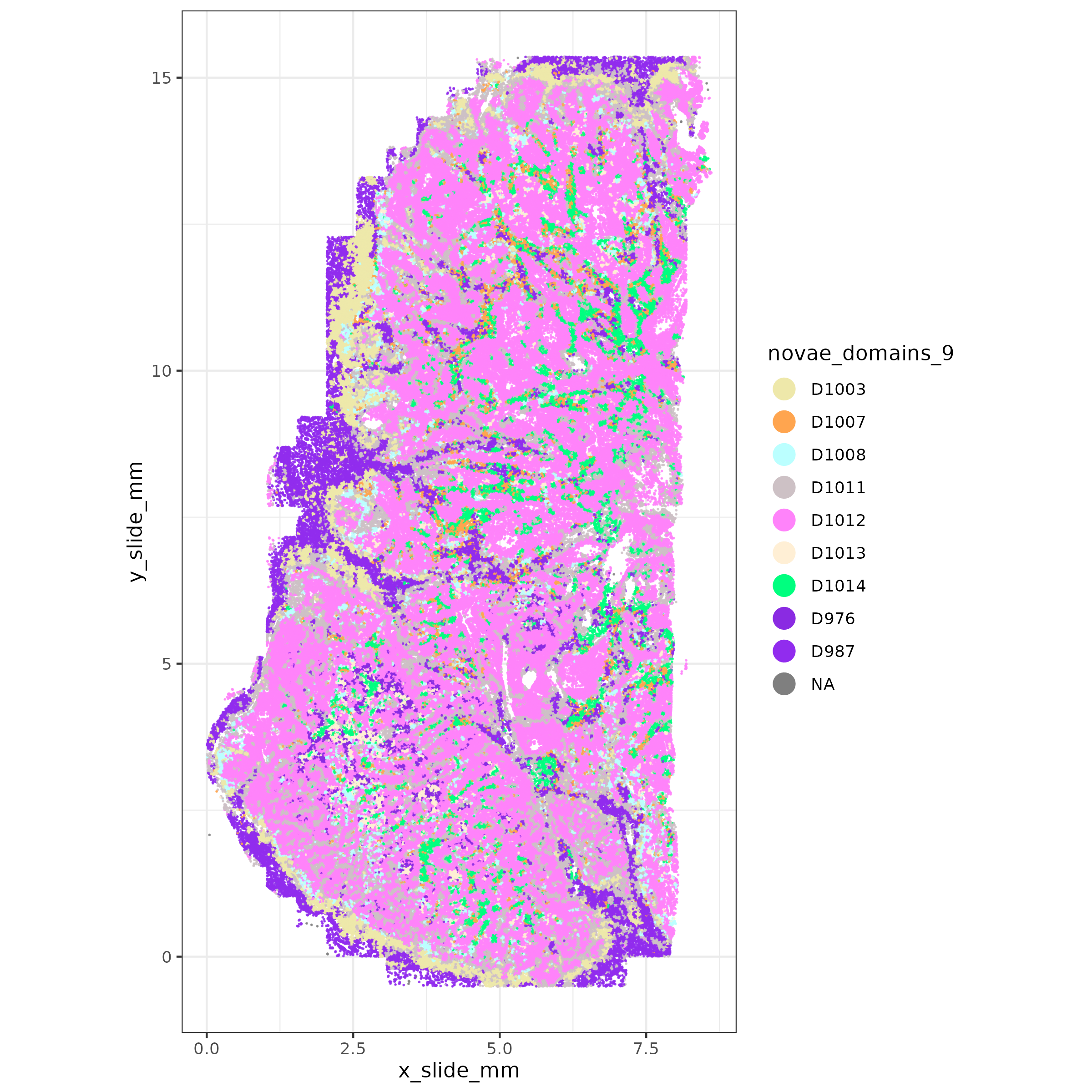
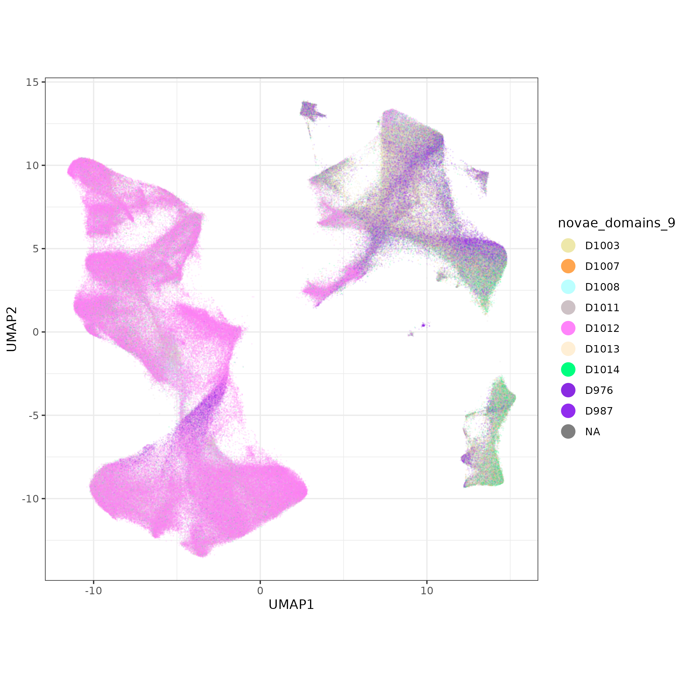
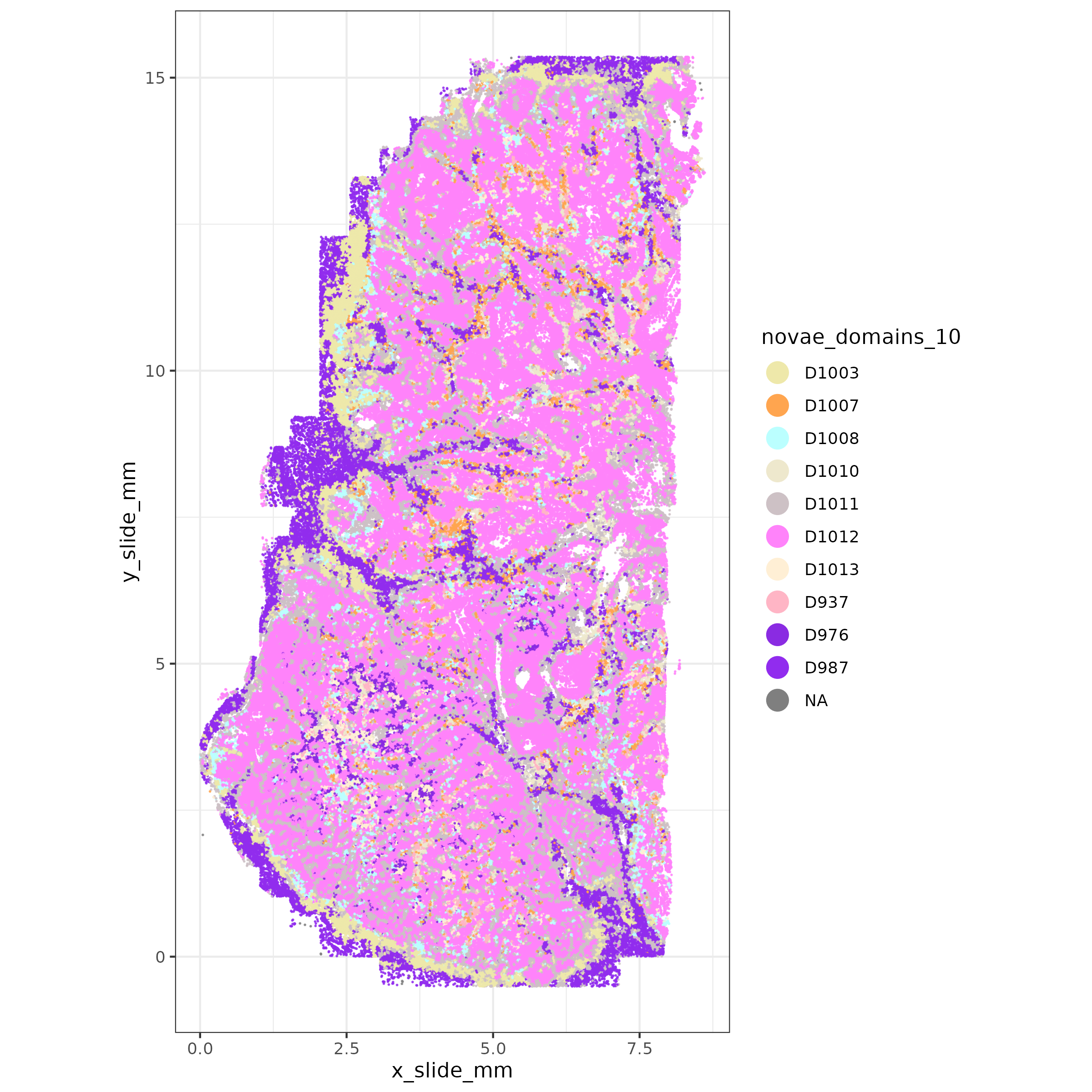
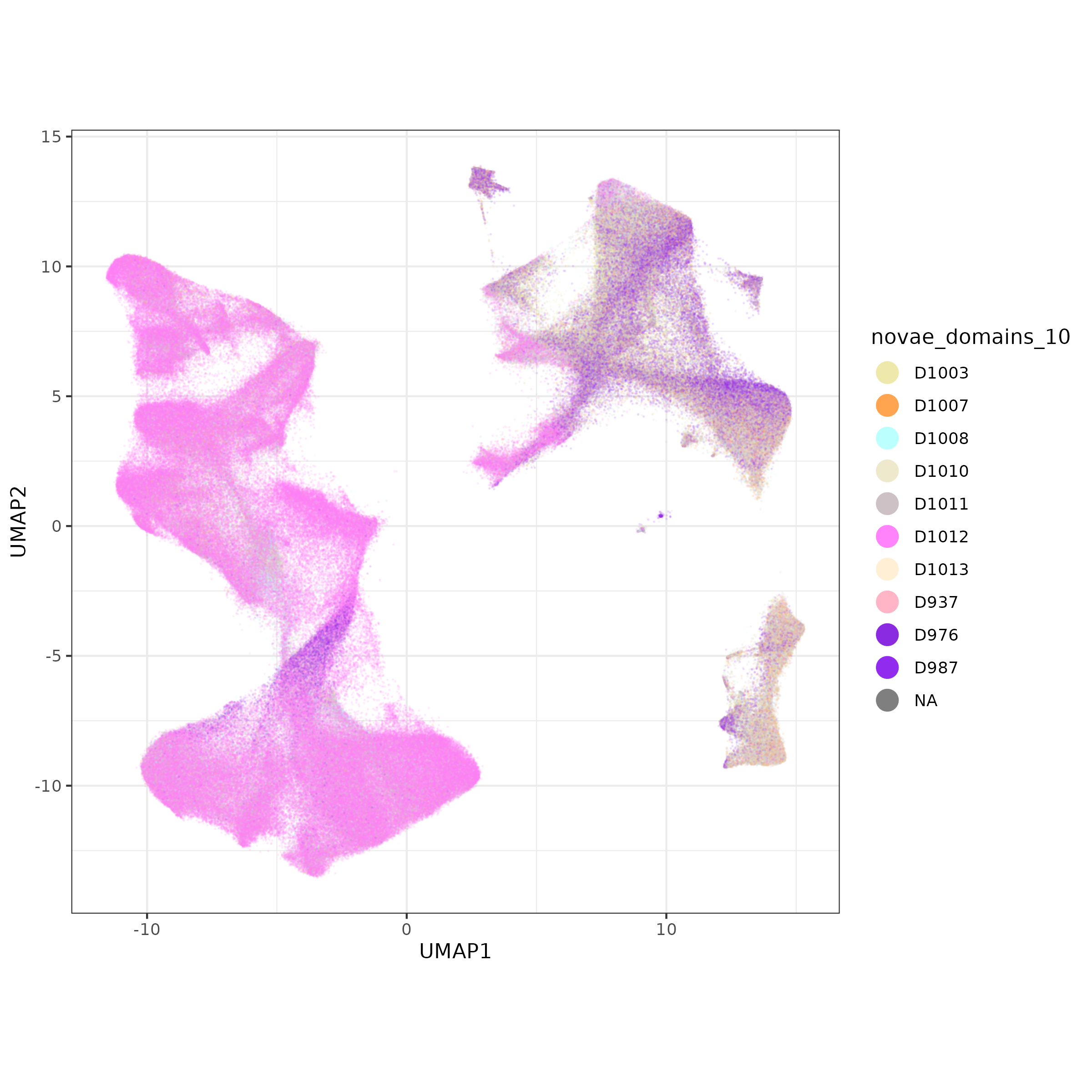
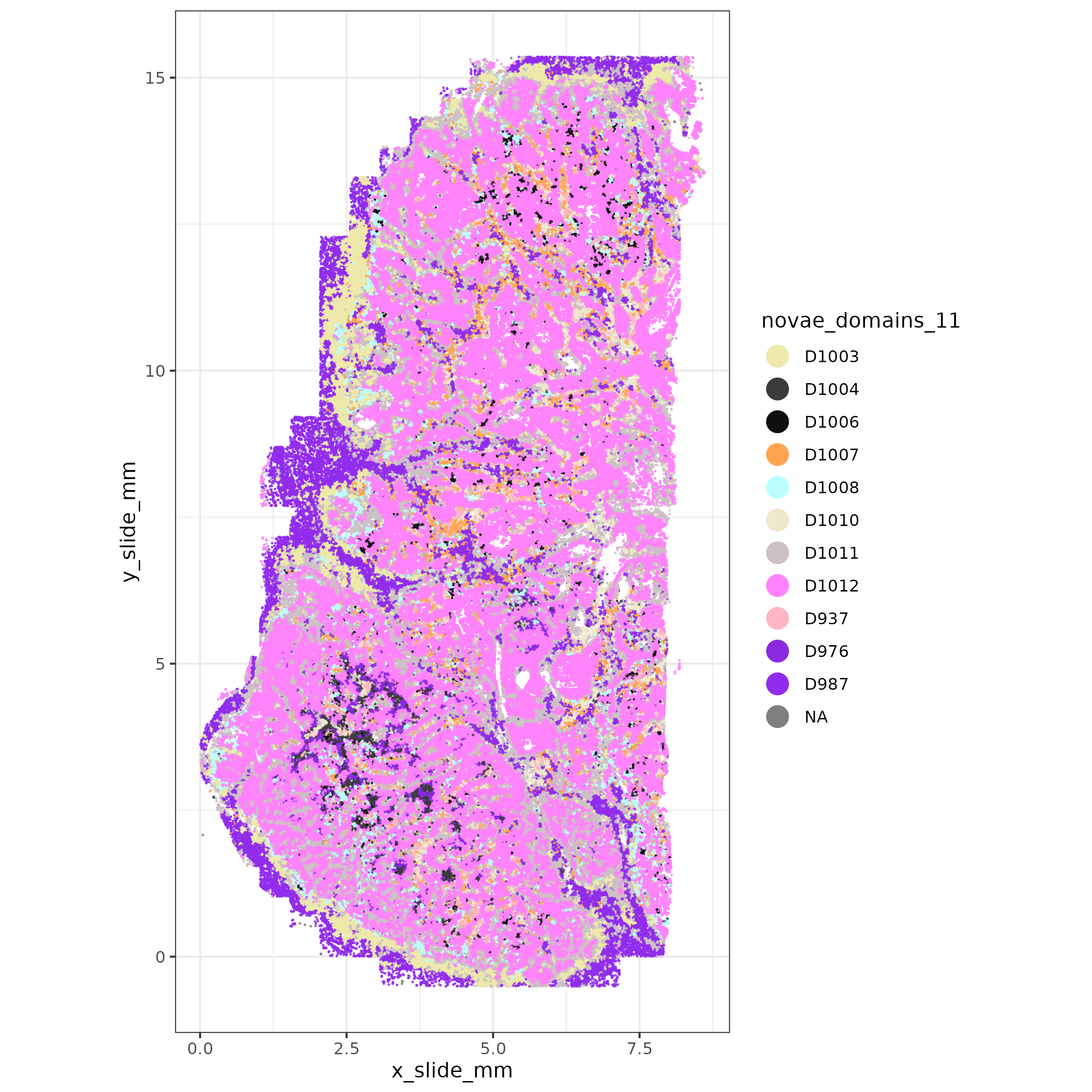
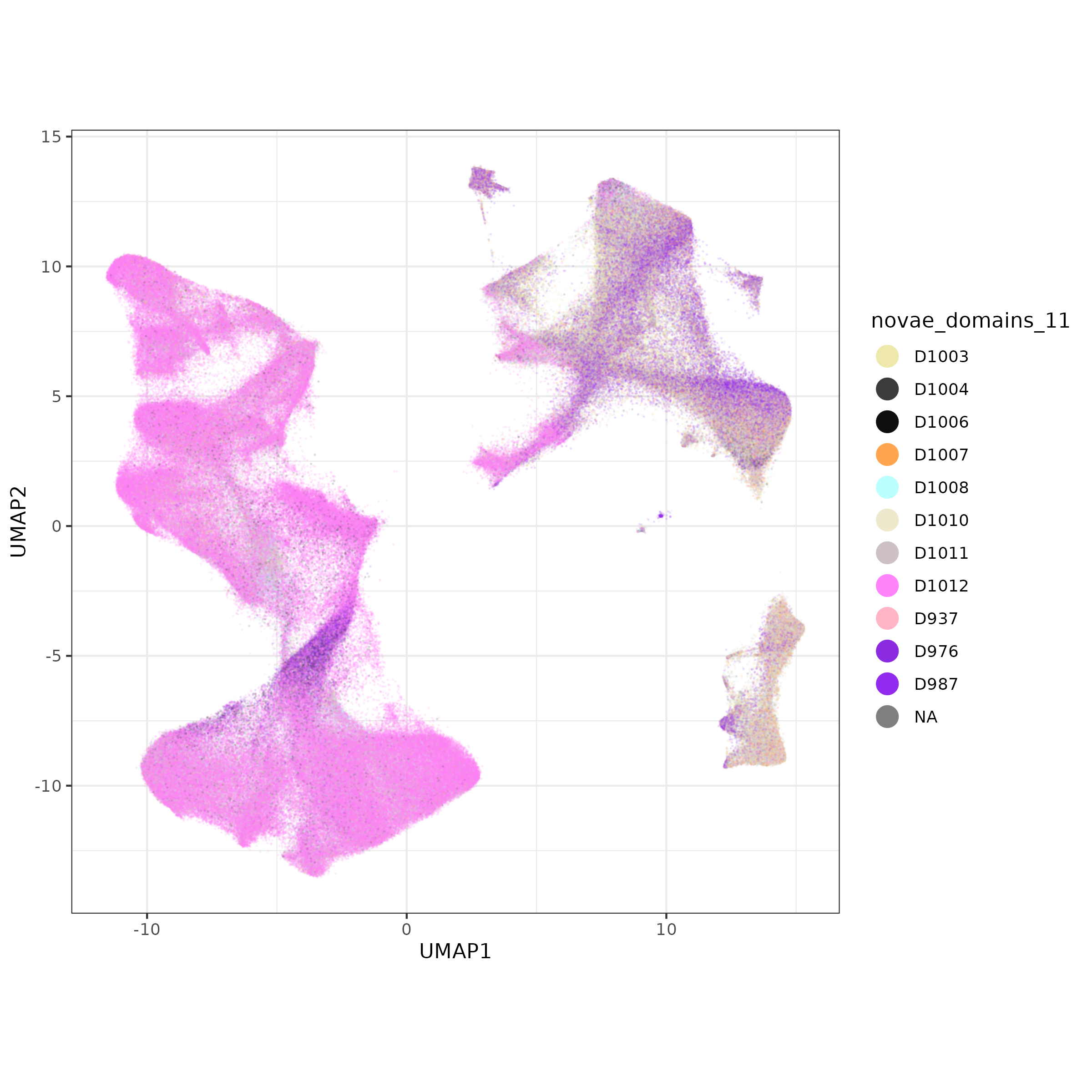
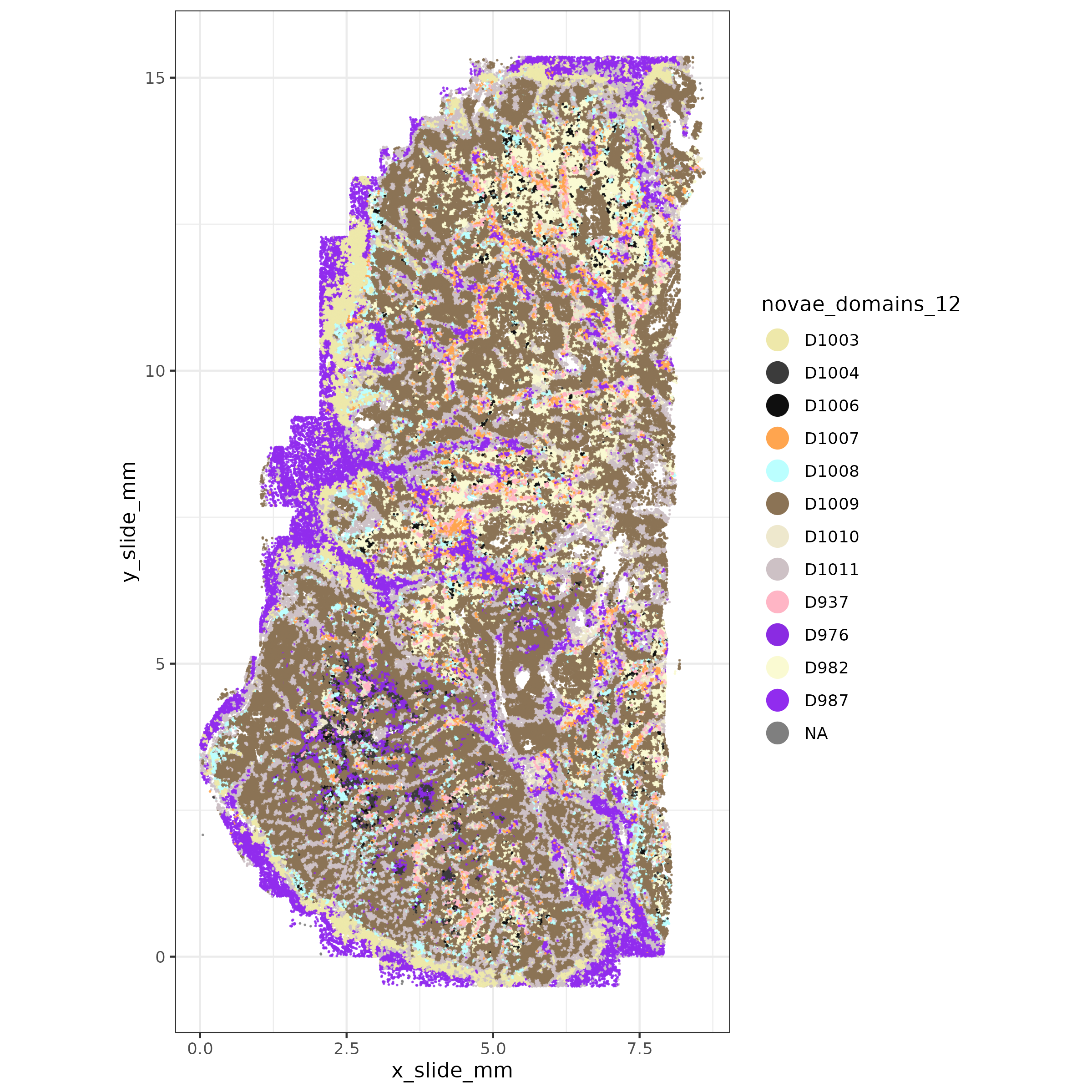
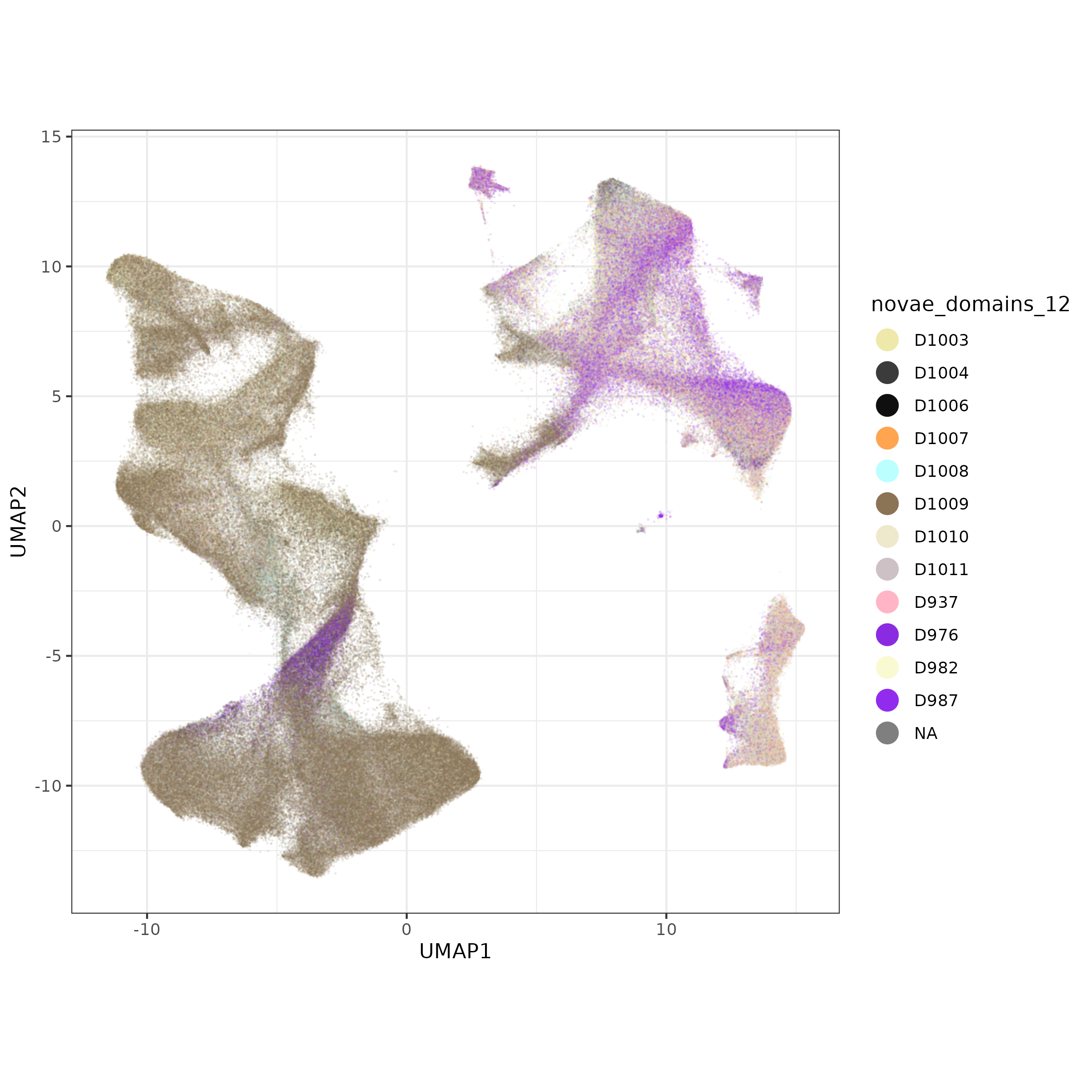
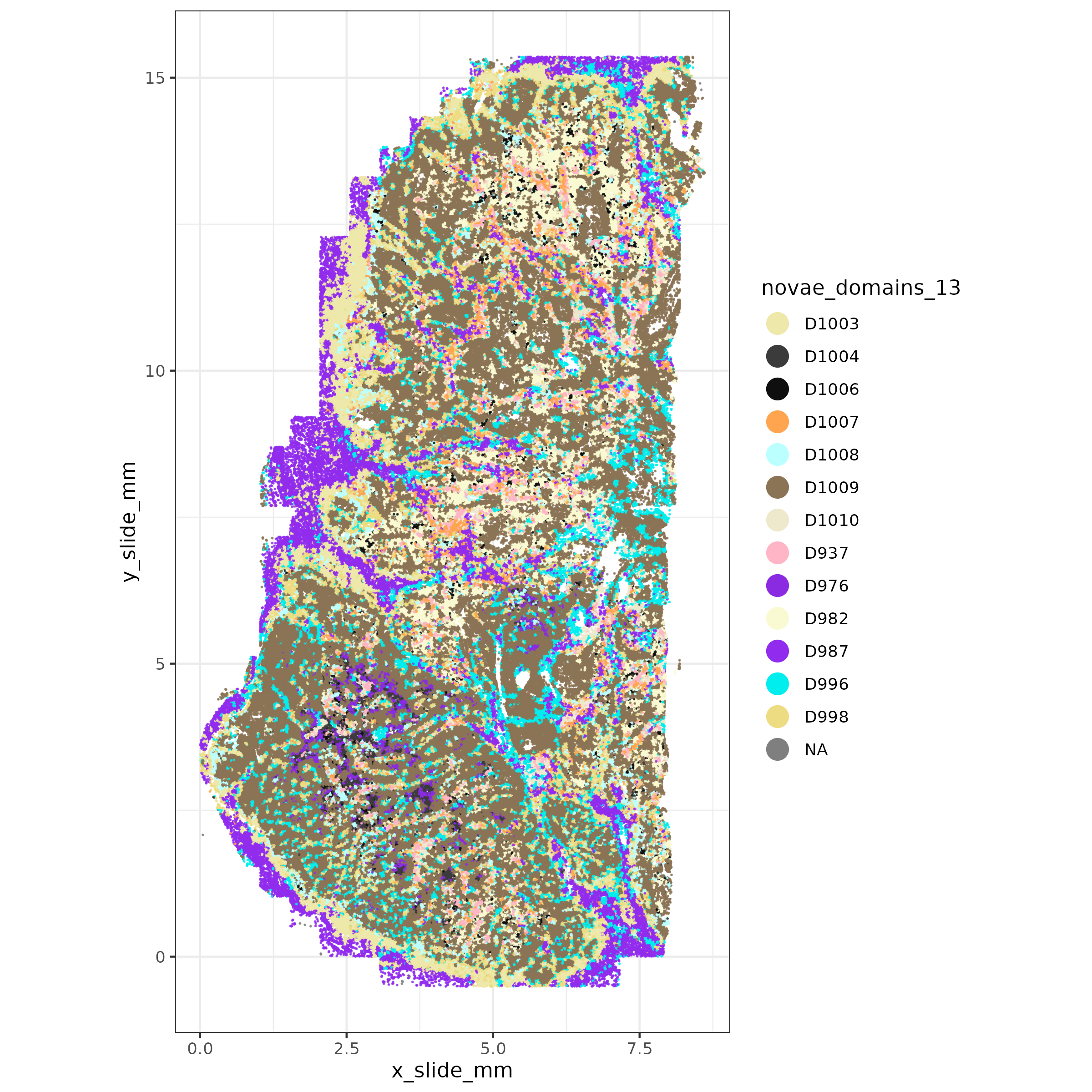
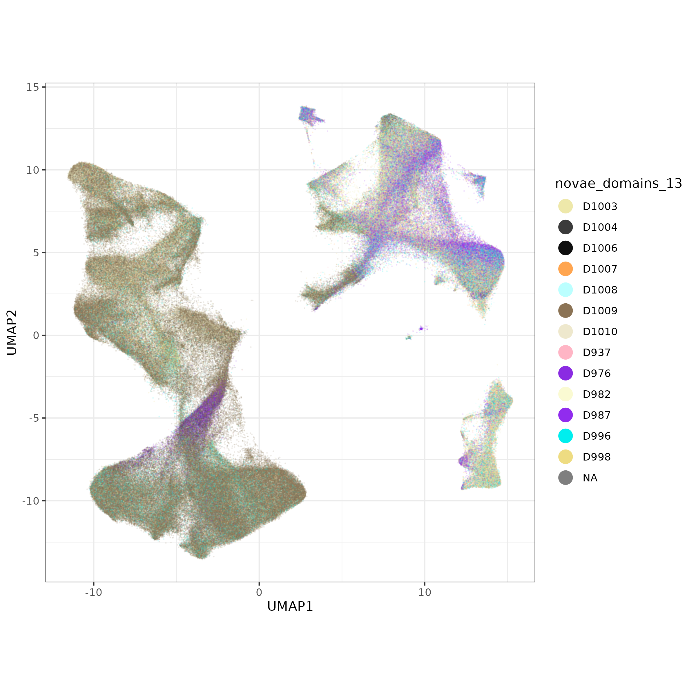
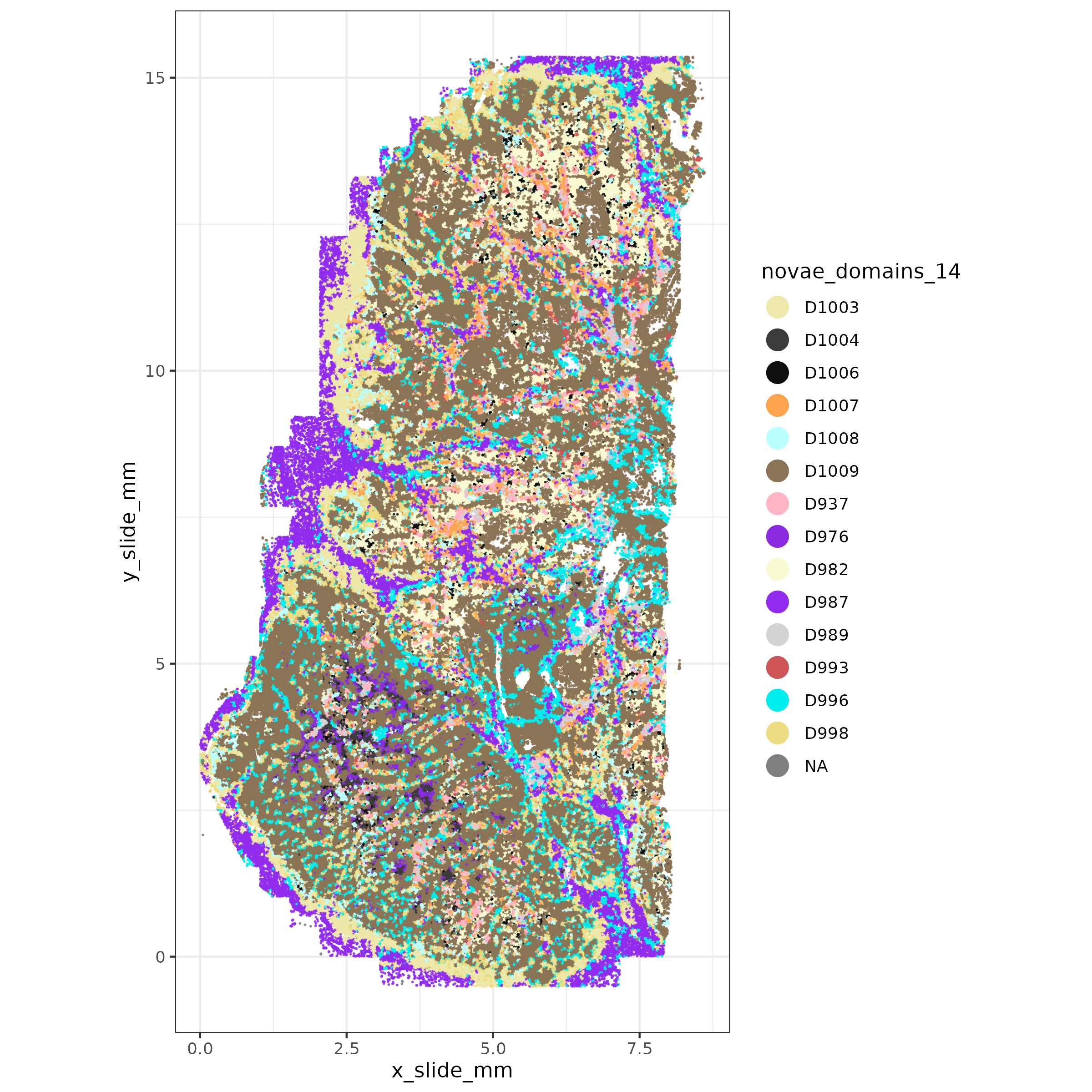
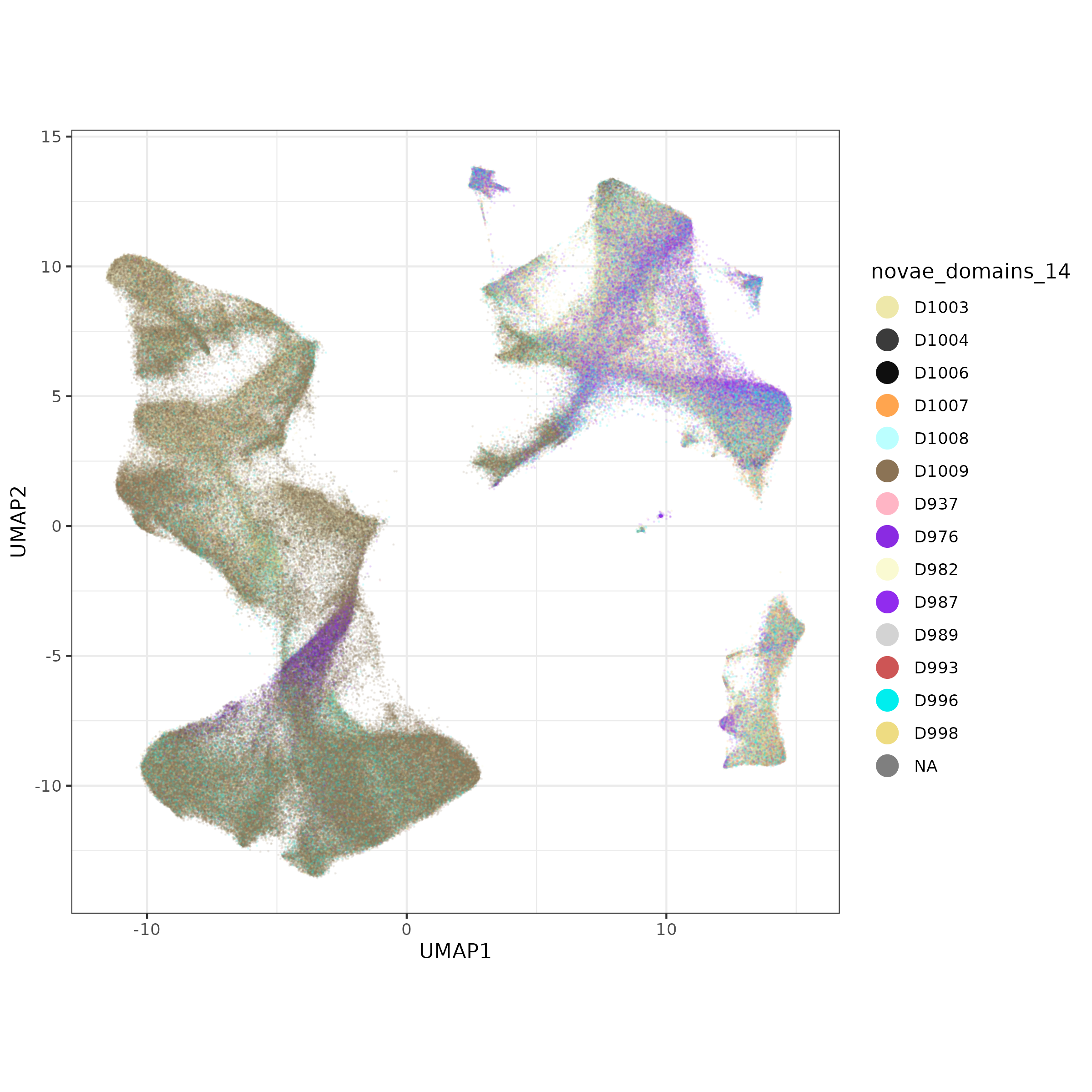
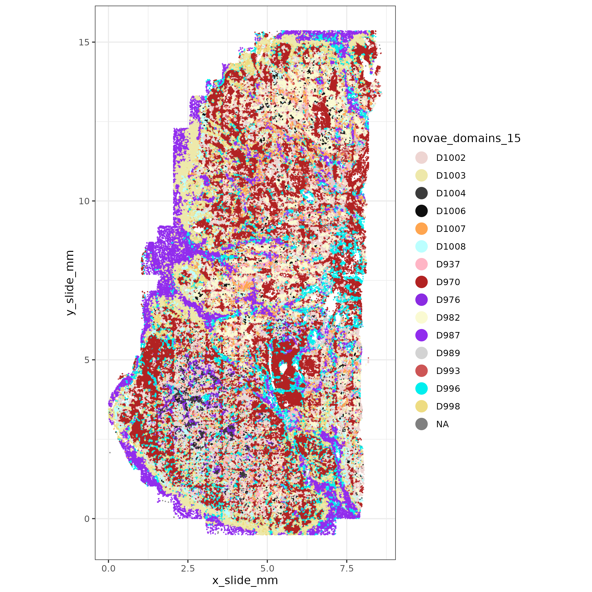
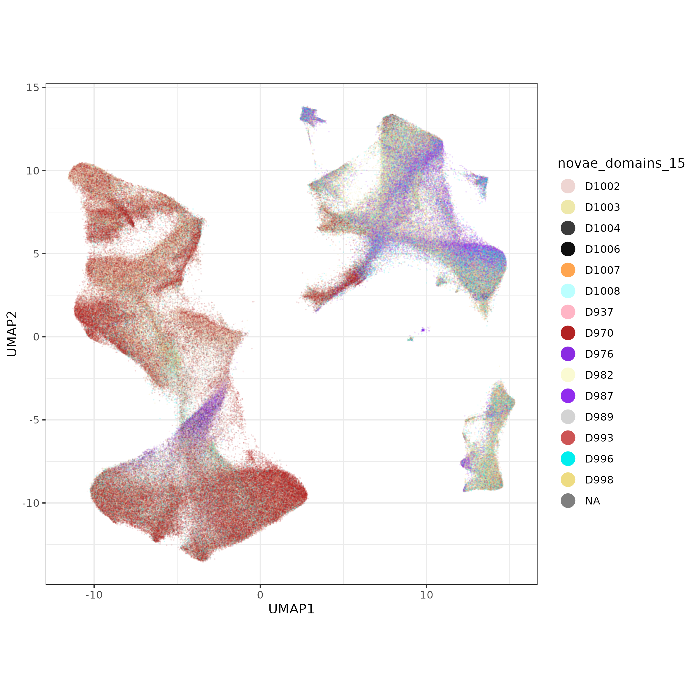
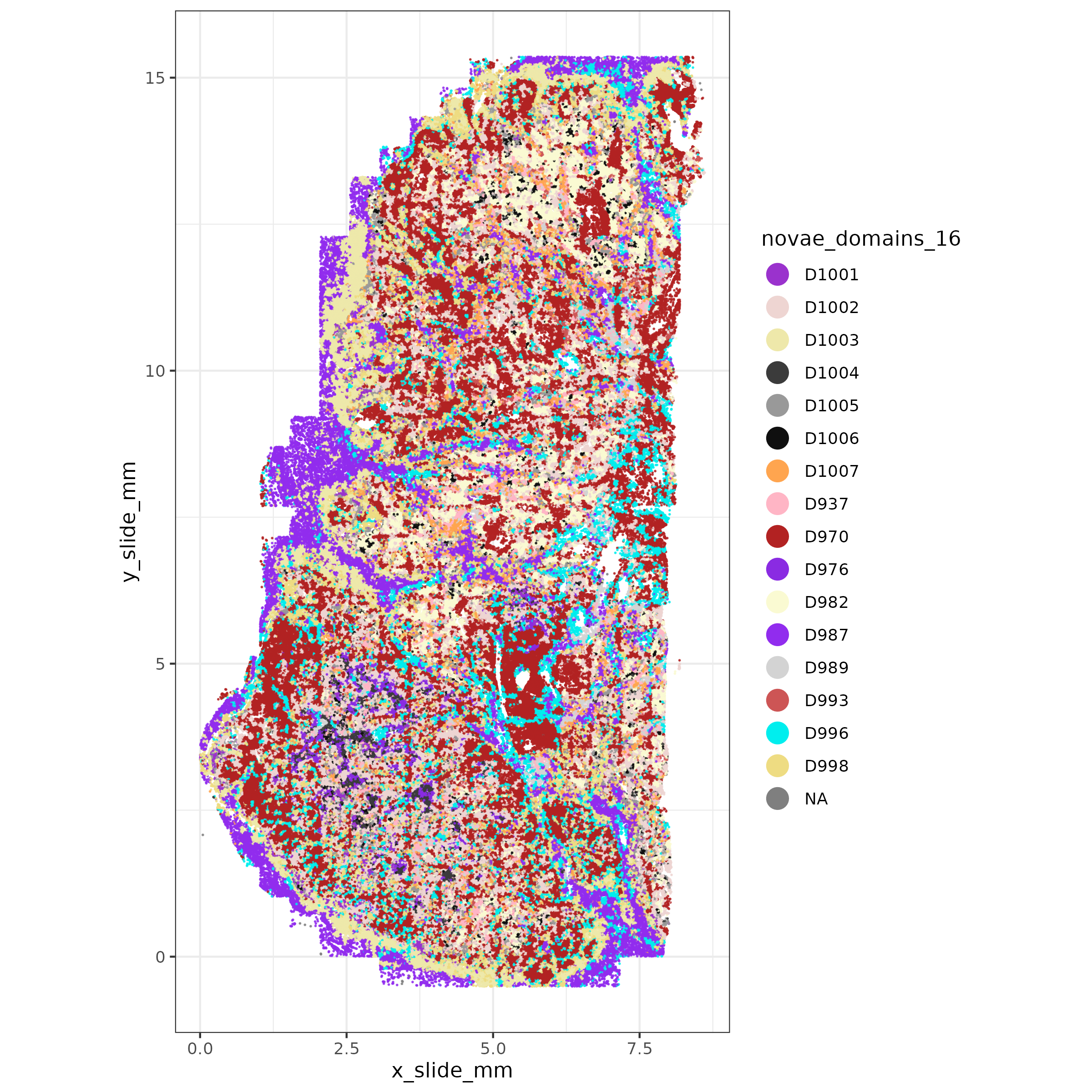
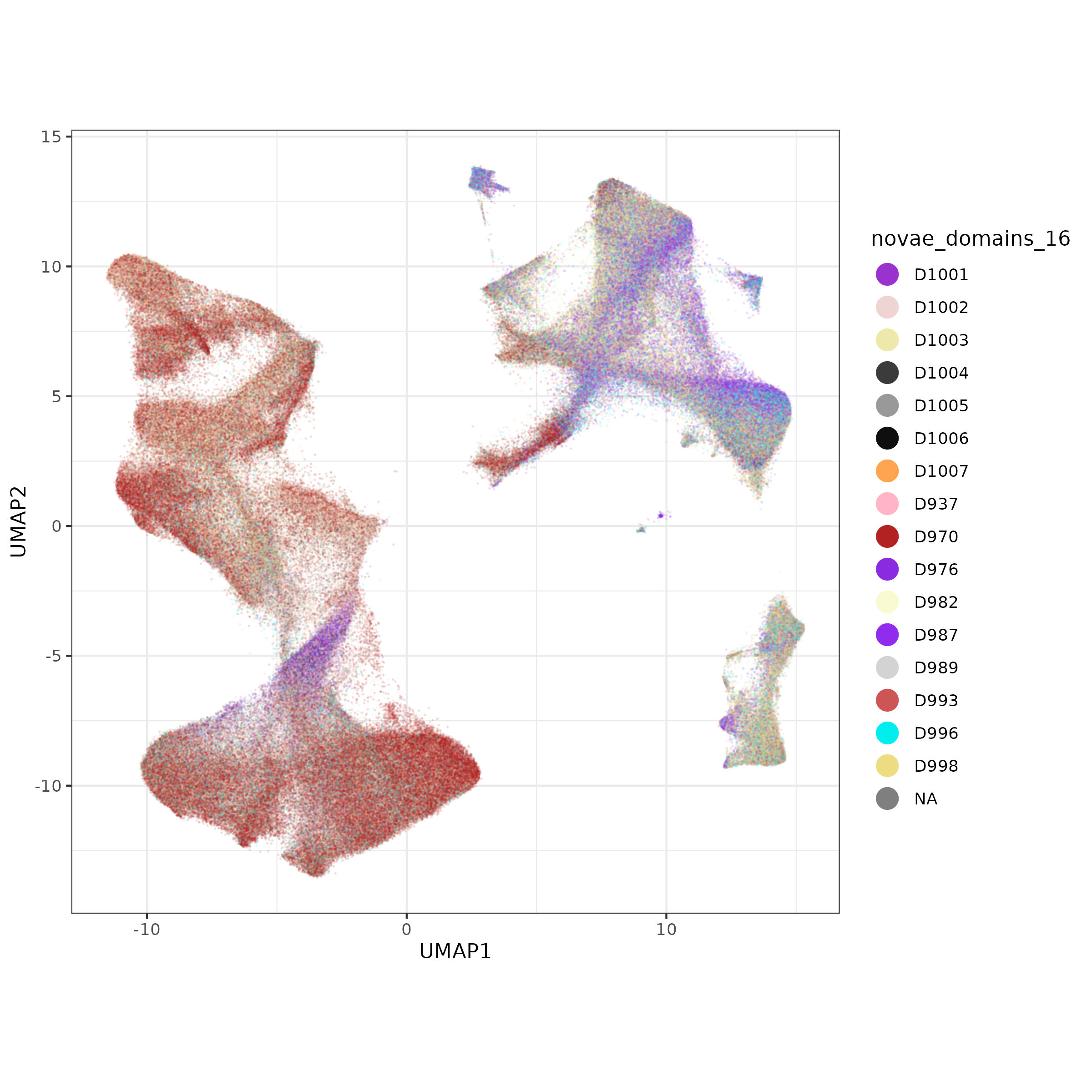
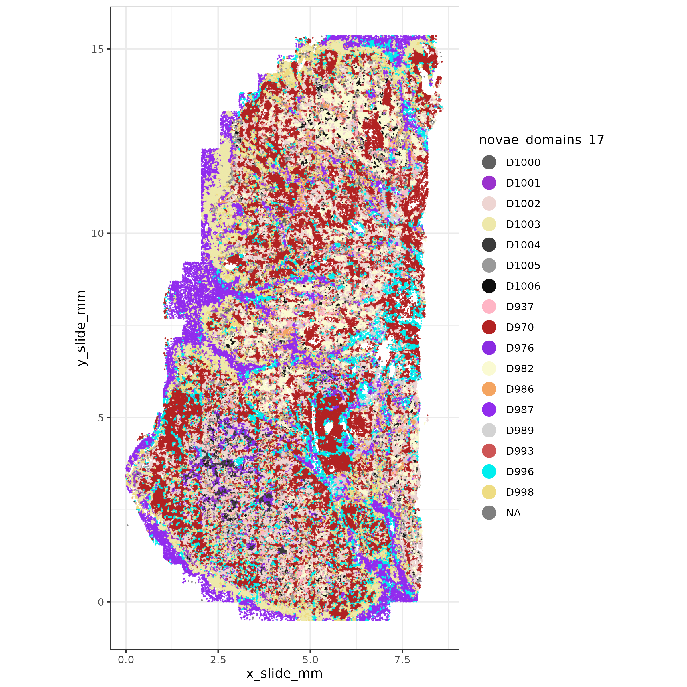
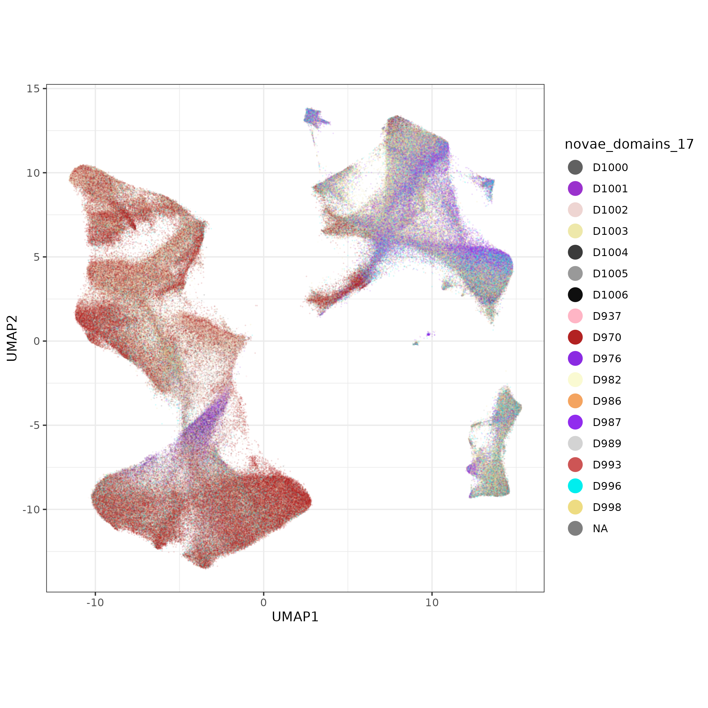
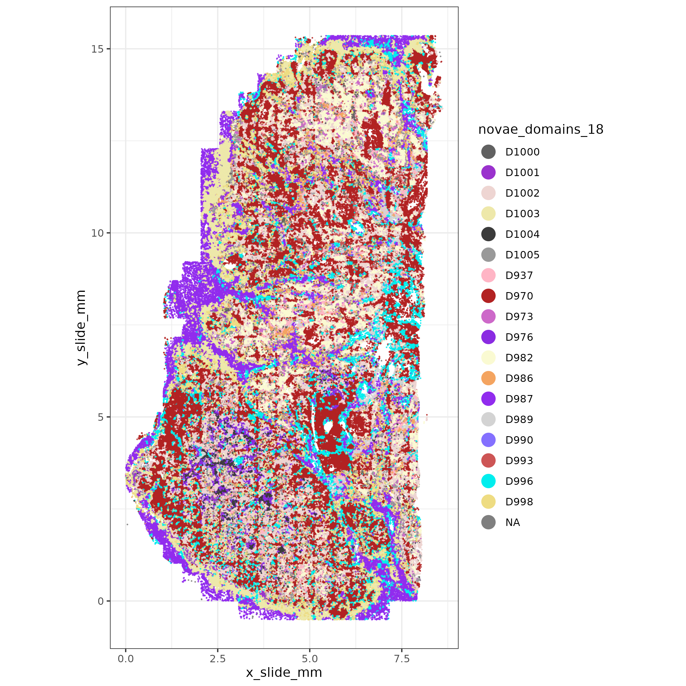
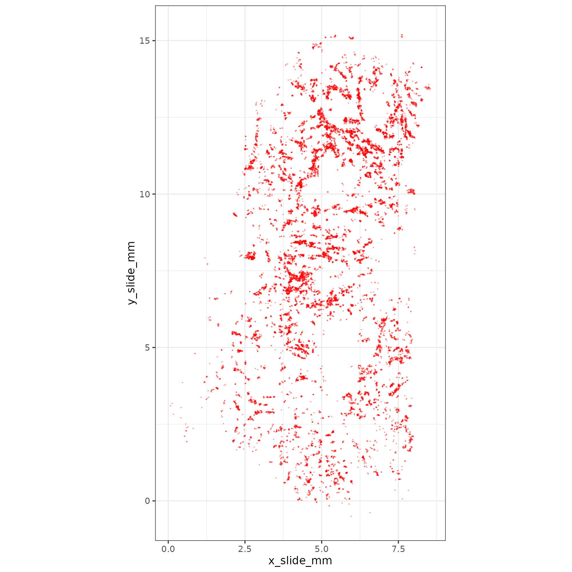
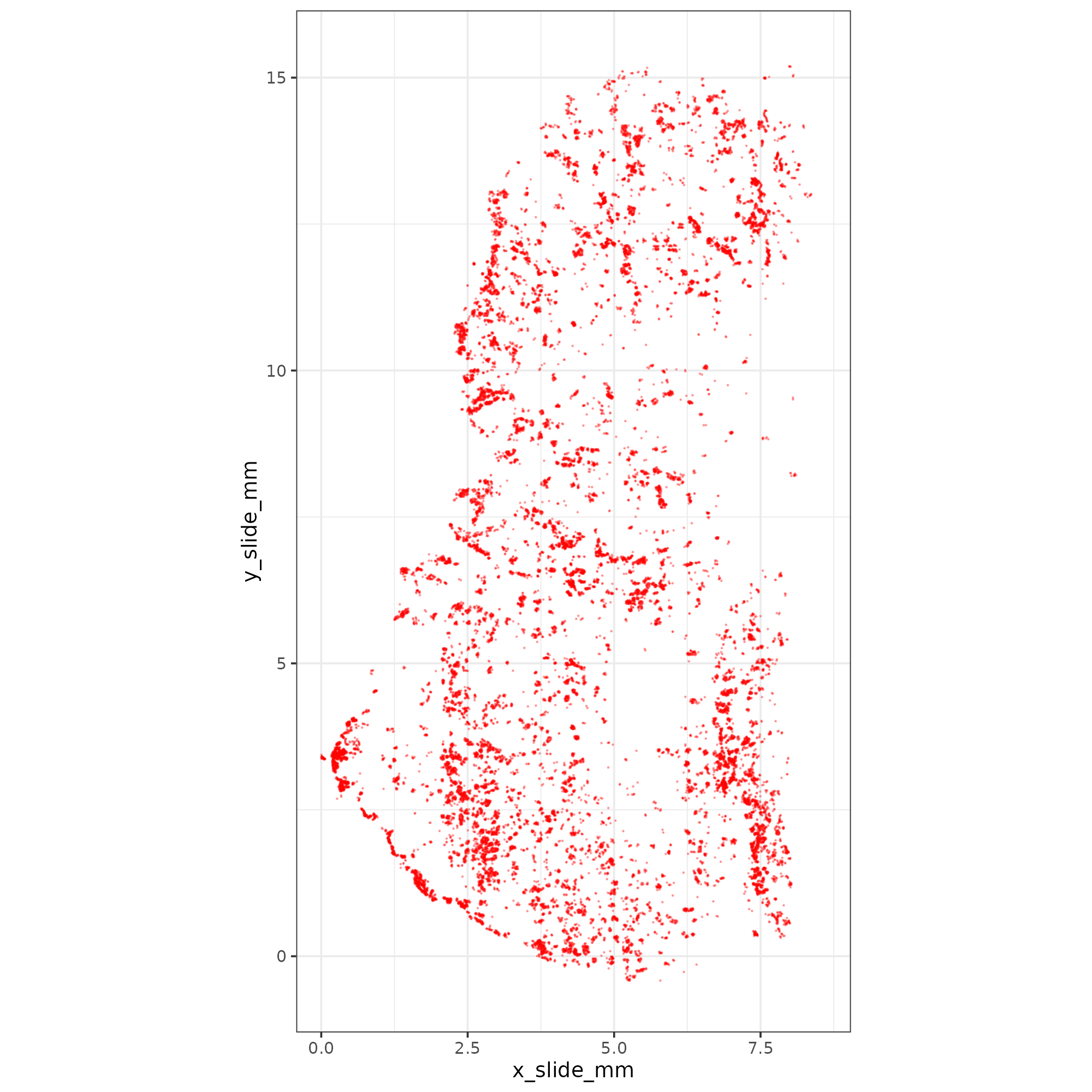
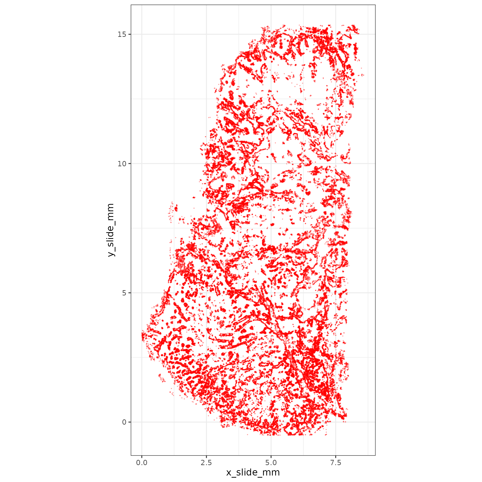
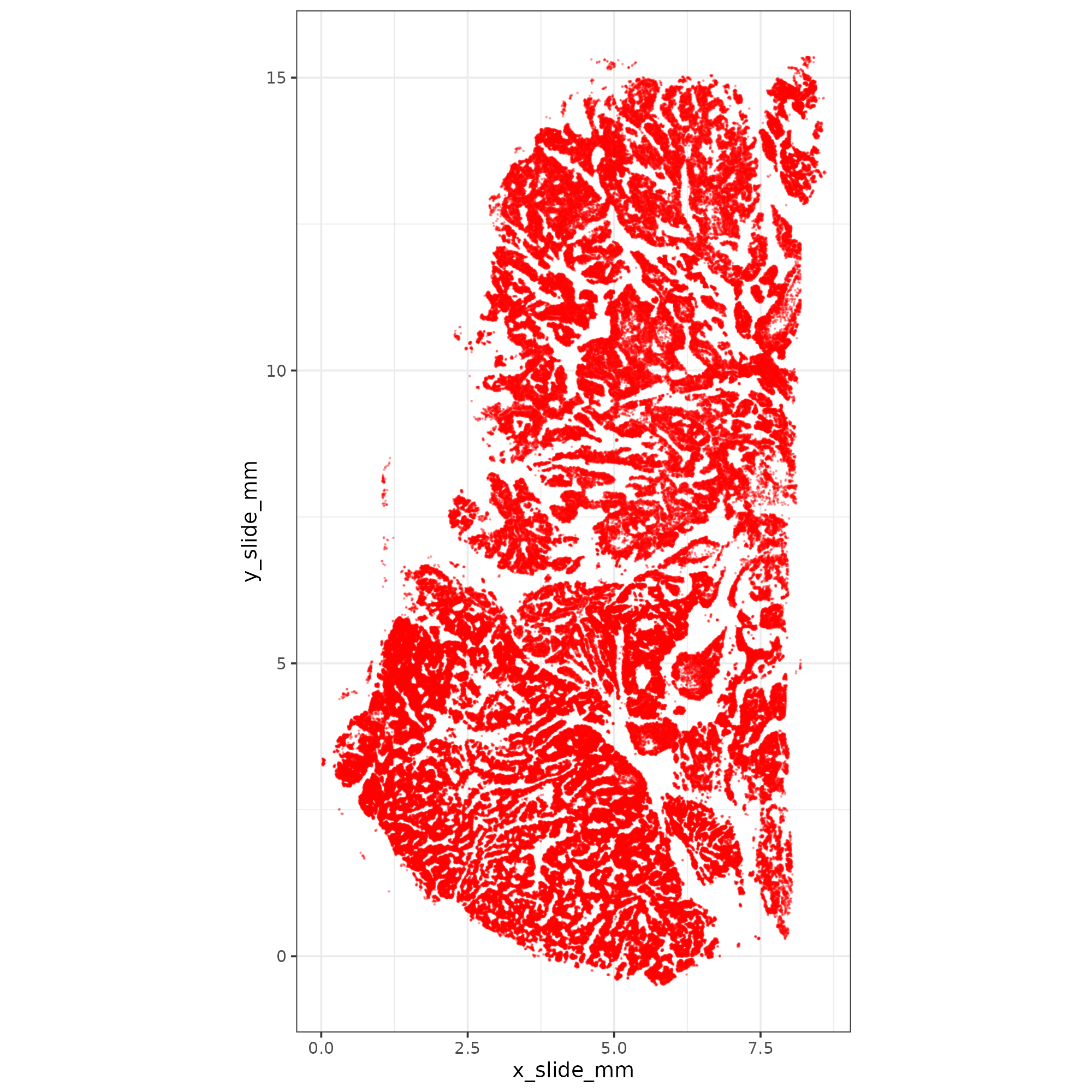
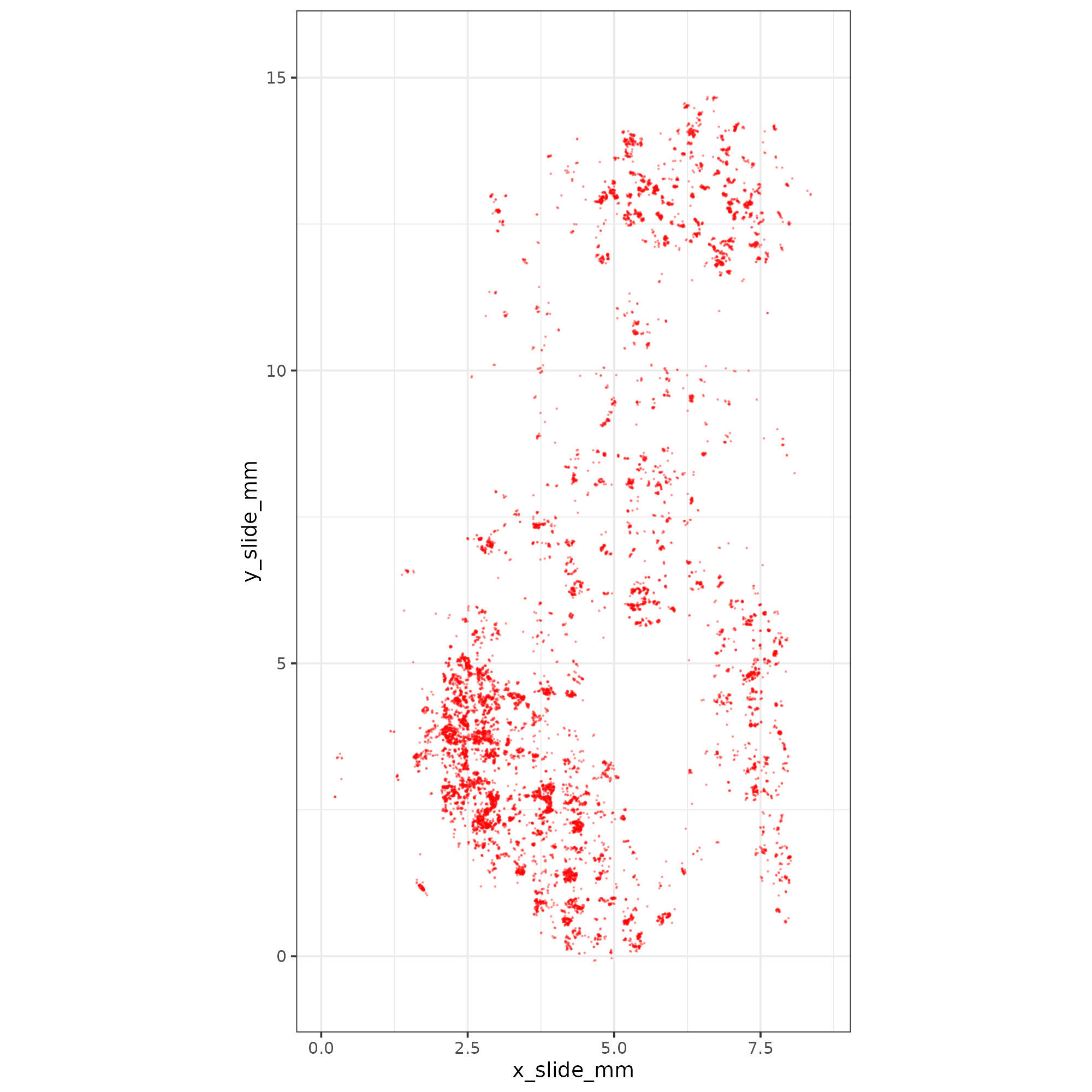
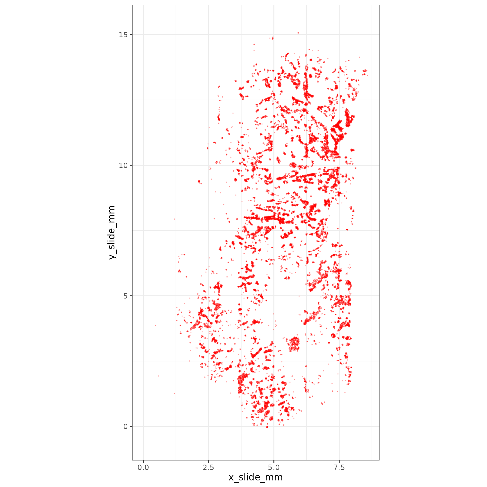
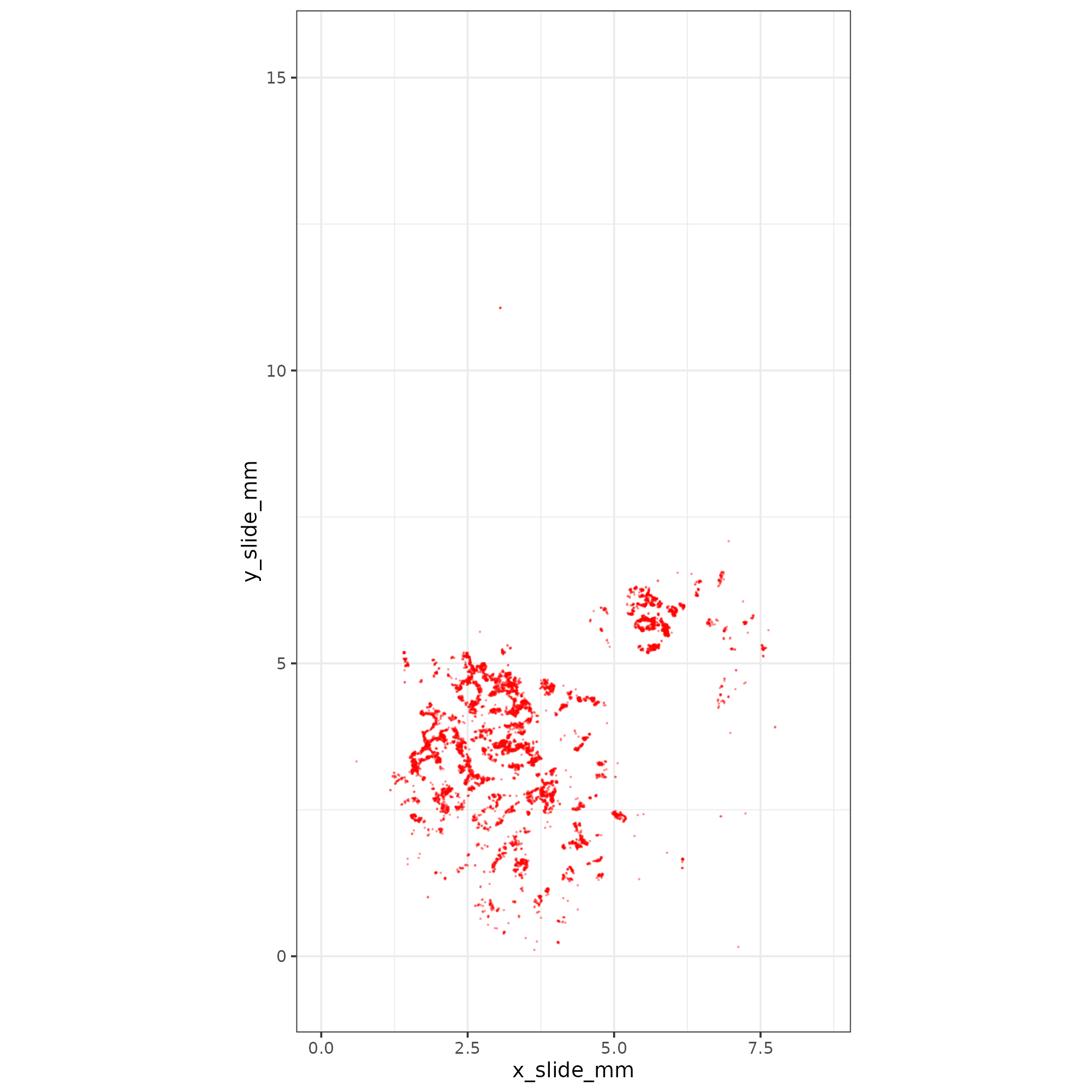
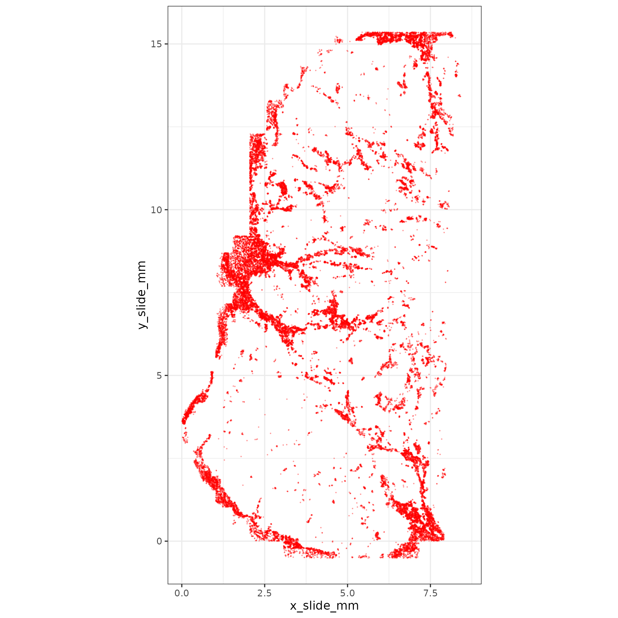
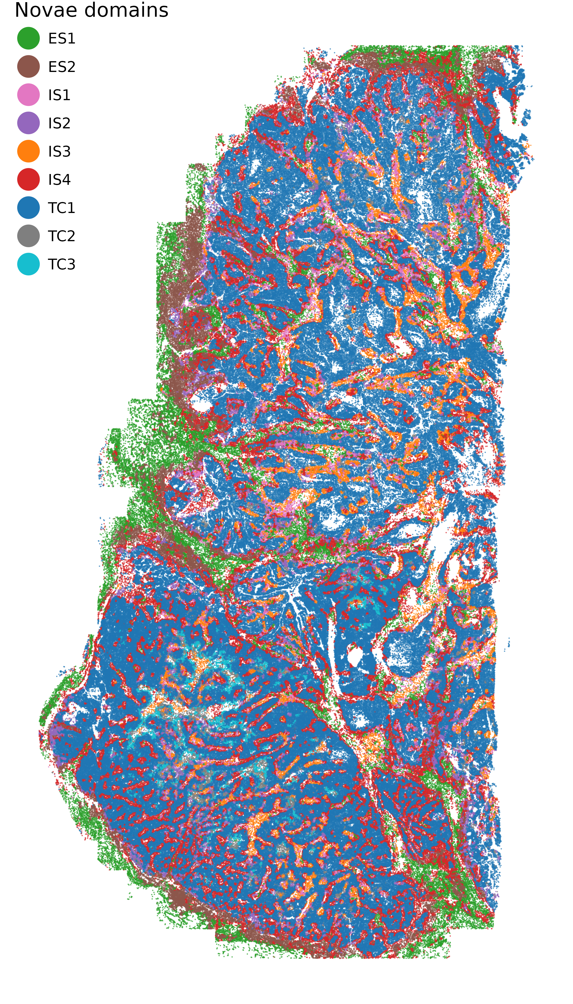
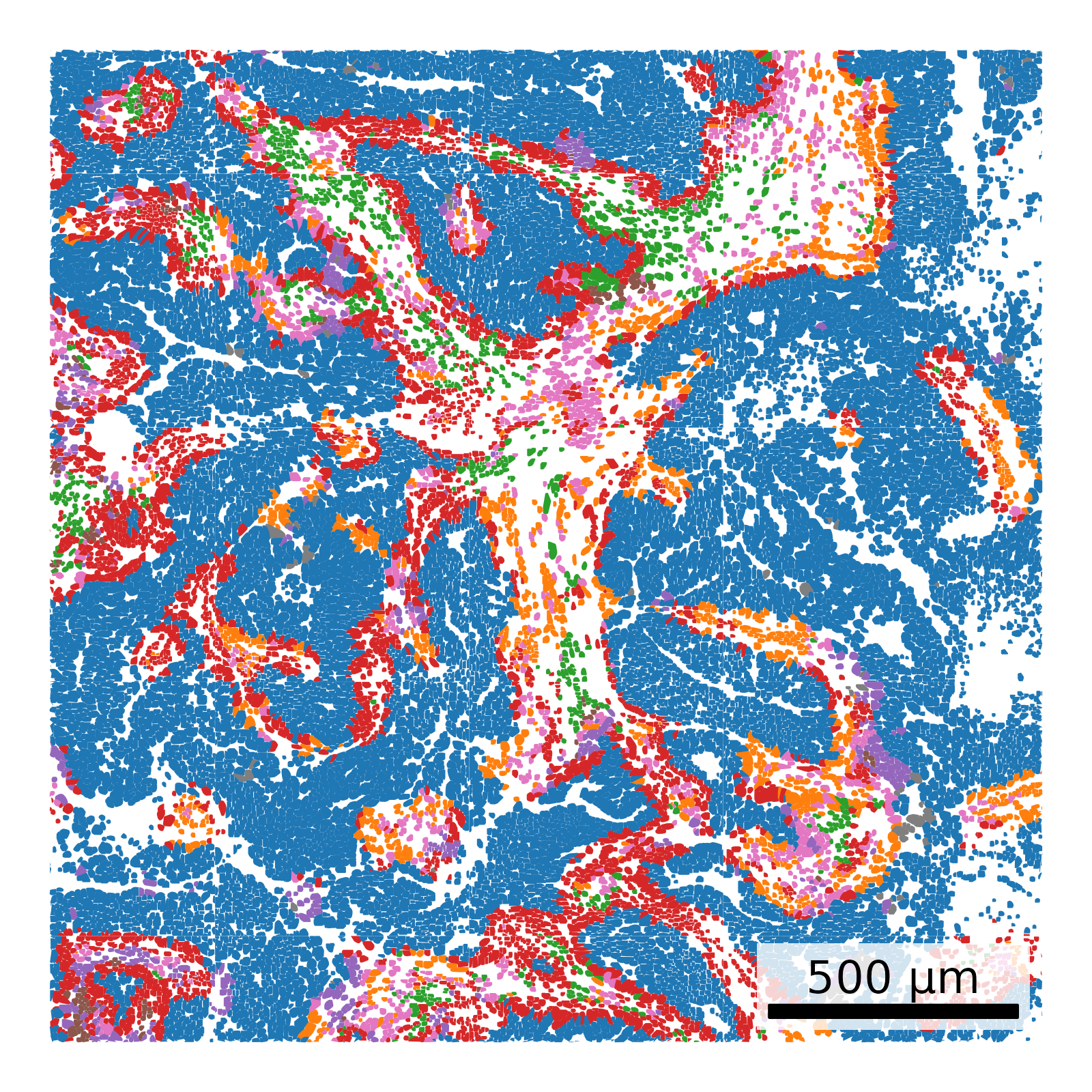
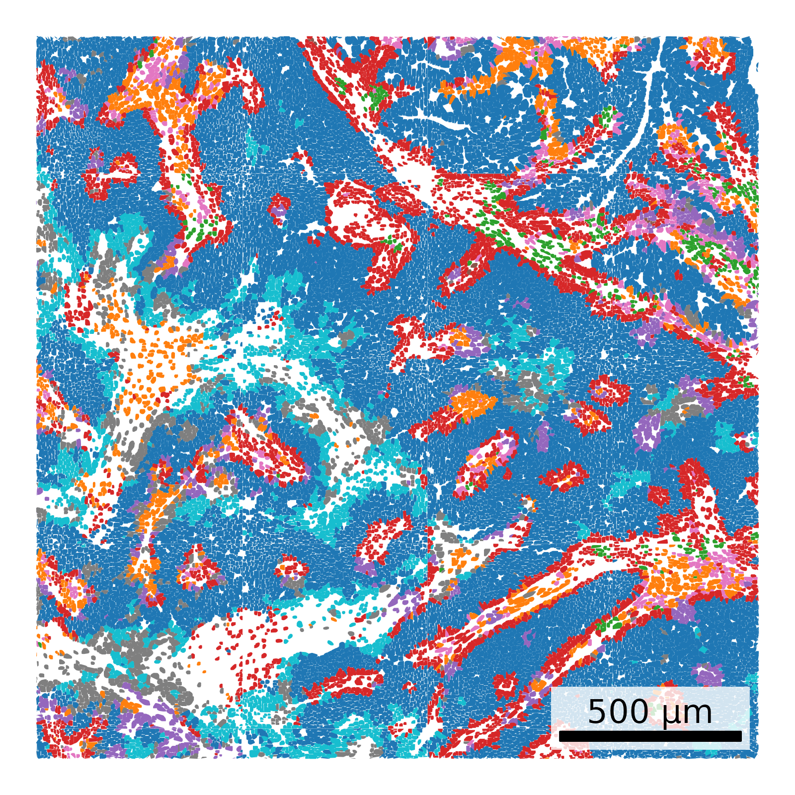
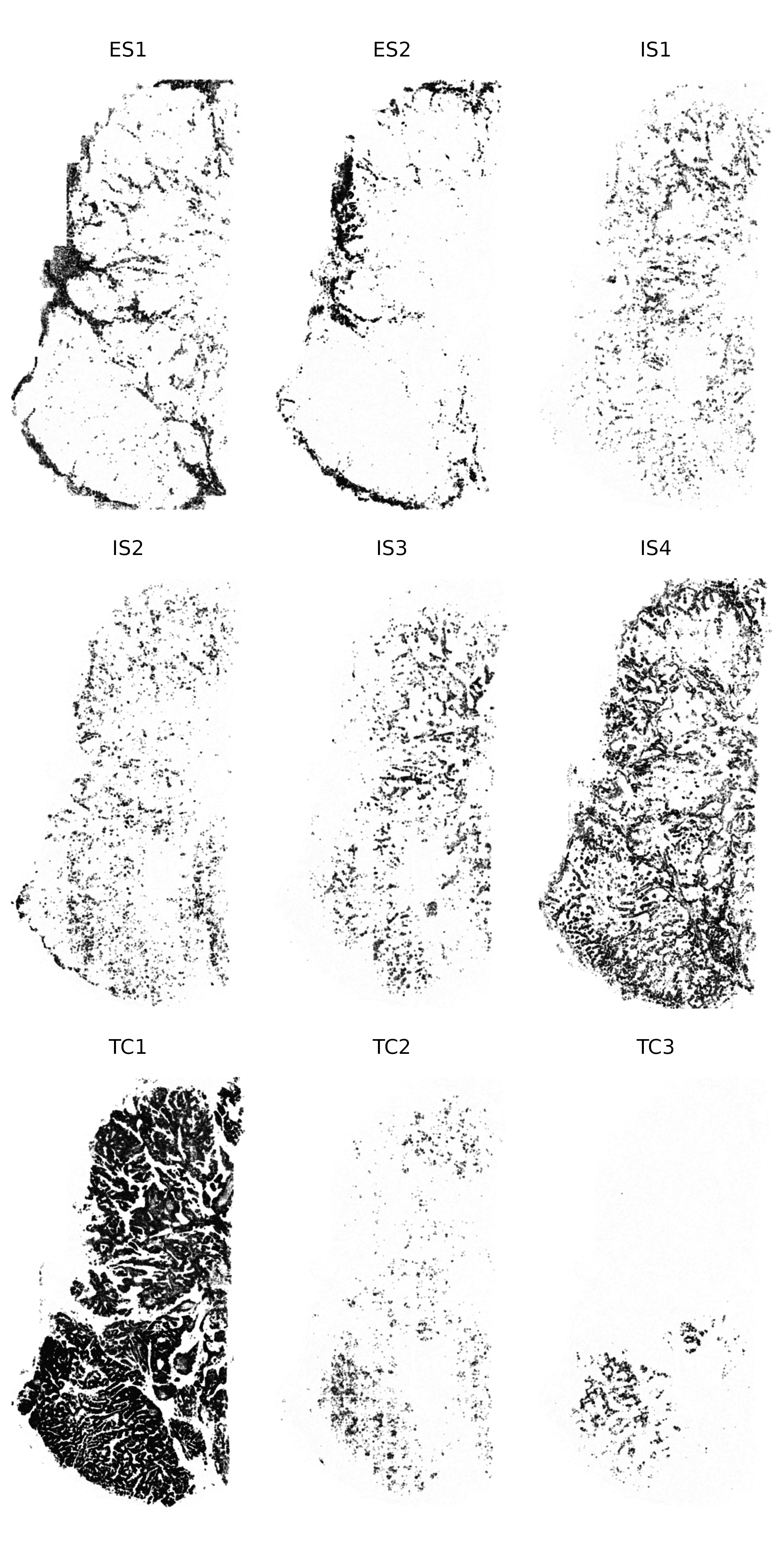
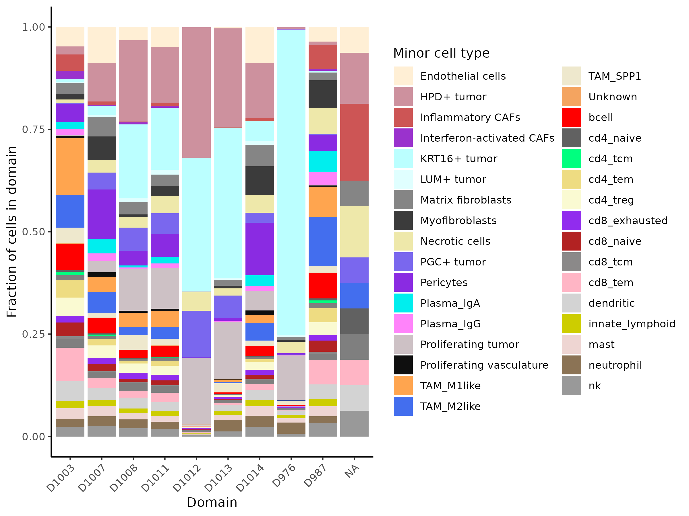
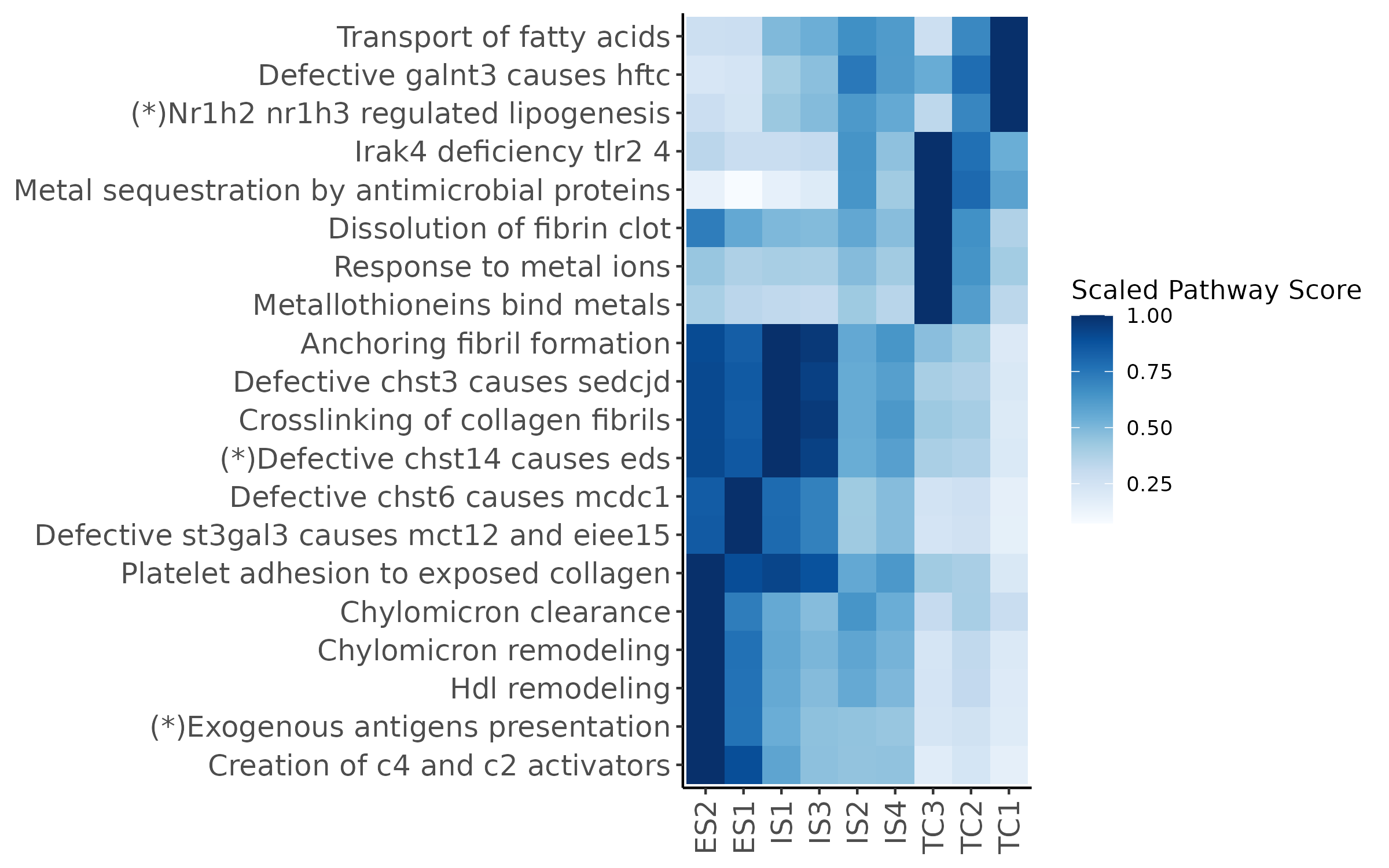
In this section, we use Novae to identify spatial domains within this dataset.

As this package is written in python, we start by generating an adata object from our filtered Seurat object.

# if there's no seurat object, read it in
if (!("seu.obj" %in% ls())){
  seu.obj <- readRDS(results_list$seurat_file_postCellTyping)
}

# Convert to single cell experiment
sce <- as.SingleCellExperiment(seu.obj)

# Save as h5ad
h5ad_path <- paste0(objects_dir, "/assay_data.h5ad")
writeH5AD(sce, file = h5ad_path, X_name = "counts", assay = "counts")

Next, we switch into Python and run novae to generate spatial domains.

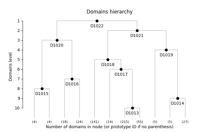
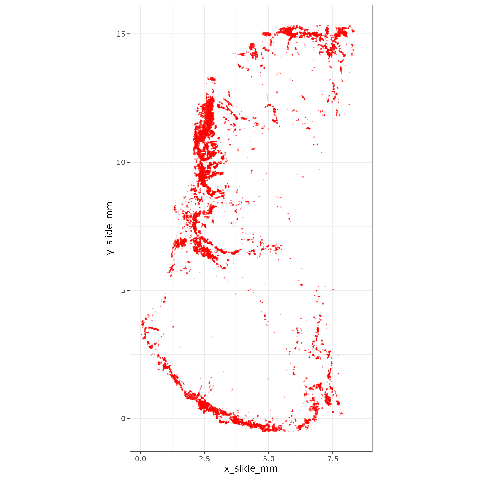
import novae
import igraph
import matplotlib
matplotlib.use('Agg')
import matplotlib.pyplot as plt
import scanpy as sc
import numpy as np
import os
import hdf5plugin

sc.settings.figdir = os.path.join(r.niche_dir, "Plots")
novae.settings.auto_preprocessing = True


# Read in sample
adata = sc.read_h5ad("analysis/Robjects/assay_data.h5ad")

## convert spatial from mm to microns for novae

# Extract coordinates from obs
x_mm = adata.obs["x_slide_mm"].to_numpy()
y_mm = adata.obs["y_slide_mm"].to_numpy()

# Create spatial_mm matrix
spatial_mm = np.column_stack((x_mm, y_mm))
adata.obsm["spatial_mm"] = spatial_mm

# Convert to microns
spatial_um = spatial_mm * 1000
adata.obsm["spatial_um"] = spatial_um

# Duplicate spatial_um to spatial
adata.obsm["spatial"] = spatial_um

## Start running novae
# Create a Delaunay graph of the data
novae.spatial_neighbors(adata, radius=80, coord_type='generic')

# Use a quick plot to ensure that neighbors were calculated appropriately
# Looking for very few red (unconnected) cells that are only on the edges of tissue
novae.plot.connectivities(adata)

# Load in pre-trained model
model1 = novae.Novae.from_pretrained("MICS-Lab/novae-human-0")

# Fine tune model based on CosMx data in this study
model1.fine_tune(adata, max_epochs=50, logger=True) 
model1.compute_representations(adata, zero_shot=False) 

for i in range(1, 20):
  model1.assign_domains(adata, i)

model1_dir = os.path.join(r.niche_dir, "novae_model_one")
model1.save_pretrained(save_directory=model1_dir)

import matplotlib.pyplot as plt
dh = model1.plot_domains_hierarchy()
plt.savefig(os.path.join(r.niche_dir, "Plots", "novae_model1_hierarchy.png"))
plt.close()


adata.write_h5ad(
  os.path.join(r.objects_dir, "anndata-plus-novae.h5ad"),
  compression=hdf5plugin.FILTERS["zstd"],
  compression_opts=hdf5plugin.Zstd(clevel=5).filter_options
)

Hierarchy of the domains assigned by novae:

knitr::include_graphics(paste0(niche_dir, "/Plots/novae_model1_hierarchy.png"))

Plot these novae clusters in XY and UMAP space. For this plotting, we switch back into R.

df <- py$adata$obs %>% select(cell_ID, minor_cell_type, major_cell_type, starts_with("novae_domains_"))
umap_coords <- py$adata$obsm['UMAP']
colnames(umap_coords) <- c("UMAP1", "UMAP2")
xy_coords <- py$adata$obsm['spatial_mm']
colnames(xy_coords) <- c("x_slide_mm", "y_slide_mm")
df <- cbind(df, xy_coords, umap_coords)

domain_names <- c()
for(i in c(1:20)){
  pick <- which(colnames(df)==paste0('novae_domains_', i))
  print(pick)
  domain_names <- c(domain_names, sort(unique(as.character(df[,pick]))))
}
domain_names <- unique(domain_names)

if(length(domain_names) <= 26){
domain_colors <- pals::alphabet2(length(domain_names))
} else{
  set.seed(2025)
  domain_colors <- sample(colors(distinct = T), length(domain_names))
}
names(domain_colors) <- domain_names
results_list[['novae_model_1_domain_names']] <- names(domain_colors)
results_list[['novae_model_1_domain_colors']] <- as.character(domain_colors)
saveRDS(results_list, results_list_file)


for(i in c(1:19)){
  p <- ggplot(data=df, 
              aes(x=x_slide_mm, y=y_slide_mm, color=.data[[paste0('novae_domains_', i)]])) + 
    geom_point(size=0.01, alpha=0.8) + 
    theme_bw() + 
    coord_fixed() + 
    scale_color_manual(values = domain_colors) +
    guides(color = guide_legend(override.aes = list(size = 5, alpha=1)))
  
  ggsave(filename = file.path(niche_dir, "Plots", paste0("xy_model_1_domain_", i, ".png")), p,
       width=16, height=16)
  
  p1 <- ggplot(data=df, 
              aes(x=UMAP1, y=UMAP2, color=.data[[paste0('novae_domains_', i)]])) + 
    geom_point(size=0.005, alpha=0.1) + 
    theme_bw() + 
    coord_fixed() + 
    scale_color_manual(values = domain_colors) +
    guides(color = guide_legend(override.aes = list(size = 5, alpha=1)))
  
  ggsave(filename = file.path(niche_dir, "Plots", paste0("umap_model_1_domain_", i, ".png")), p1,
       width=8, height=8)  

}

x_range <- range(df$x_slide_mm)
y_range <- range(df$y_slide_mm)
for(i in c(1:19)){
  pick <- which(colnames(df)==paste0("novae_domains_", i))
  i_domains <- as.character(unique(df[,pick]))
  for(j in i_domains){
    if(is.na(j)){
      next
    }
    dat <- df[df[,pick]==j,]
    p_x <- ggplot() + 
    geom_point(data = dat, size=0.005, alpha=0.3,
               aes(x=x_slide_mm, y=y_slide_mm), color="red") +
    theme_bw() + 
    coord_fixed() + 
    scale_x_continuous(limits=x_range) + 
    scale_y_continuous(limits=y_range)
    ggsave(filename=file.path(niche_dir, "Plots", paste0("xy_model_1_domain_level_", i, "_domain_", j, ".png")),
         plot=p_x, width=8, height=8, dpi=250) 
  }
}

# Save 9 domain assignments to a separate file for easy access.
novae_9 <- df$novae_domains_9
names(novae_9) <- row.names(df)
saveRDS(novae_9, file = paste0(niche_dir, "/Data/novae_domains_9_assignments.rds"))

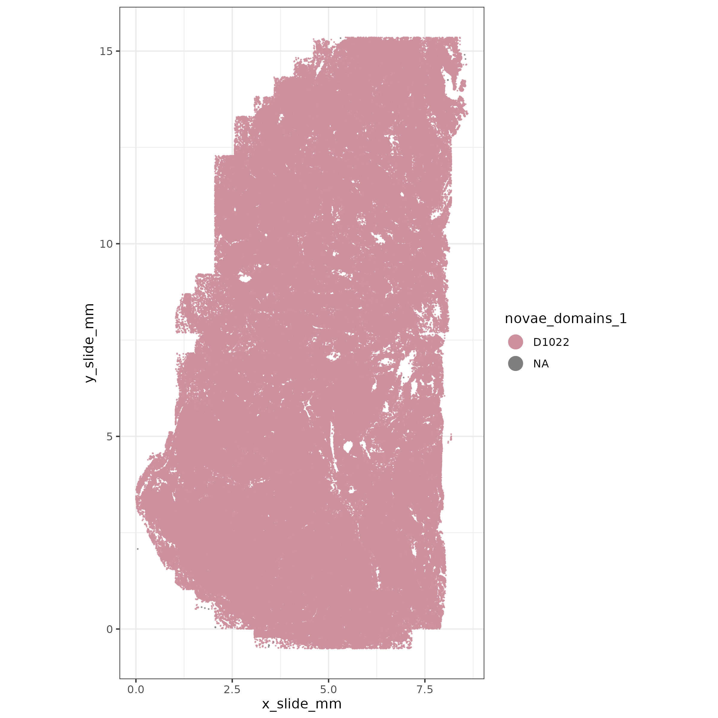
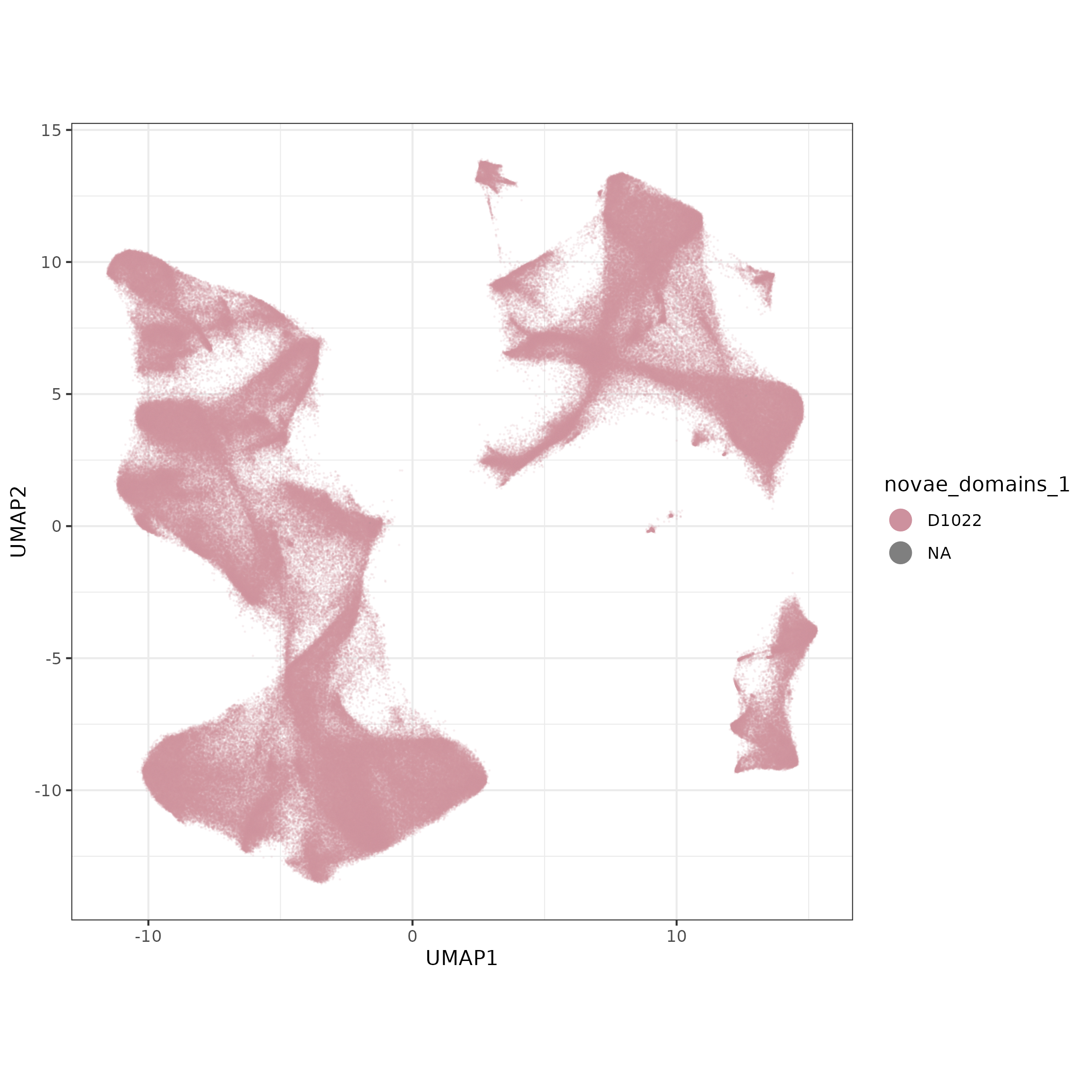
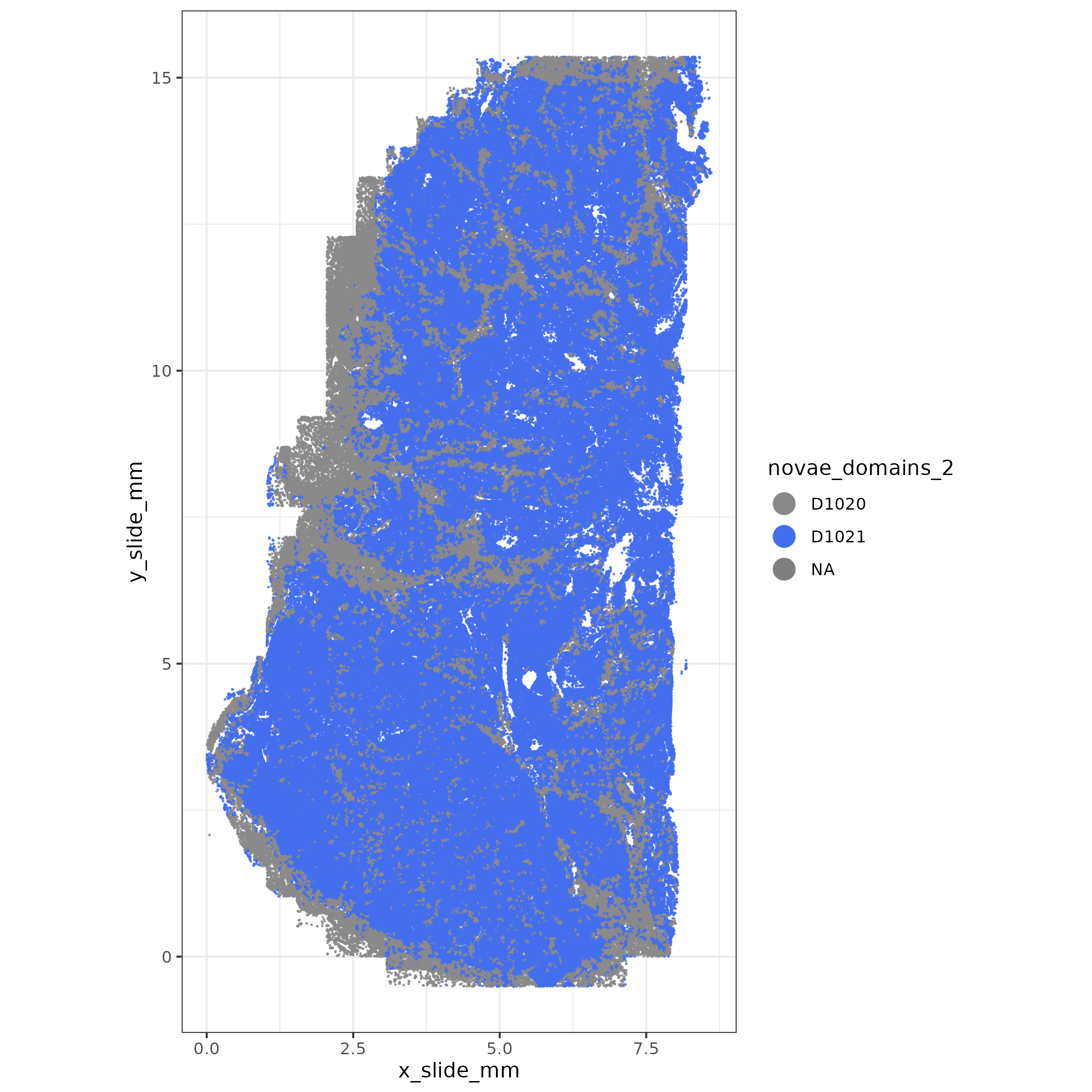
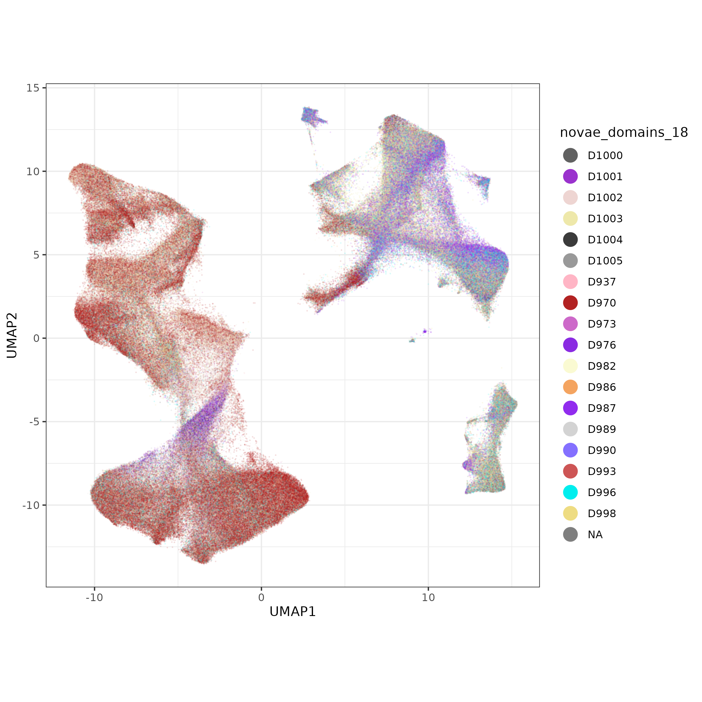
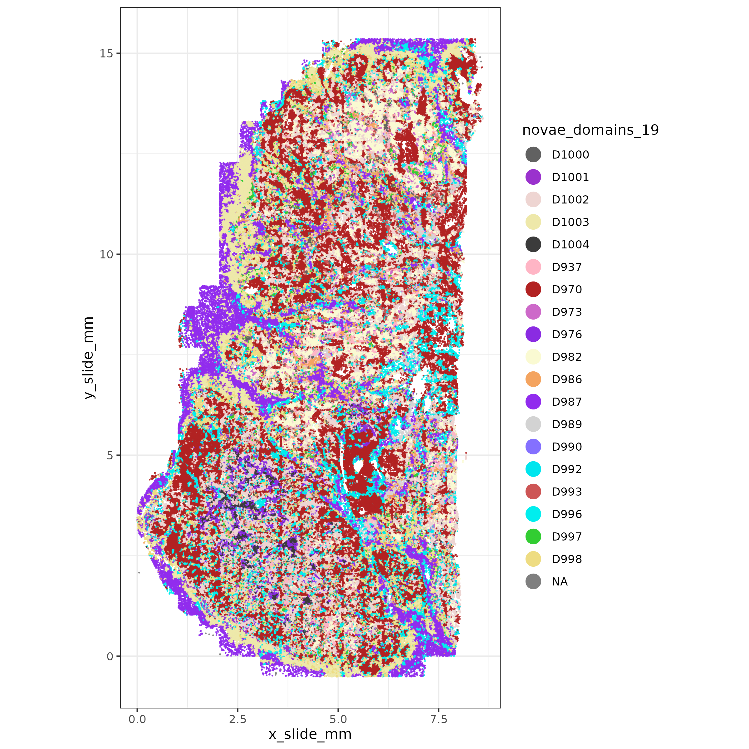
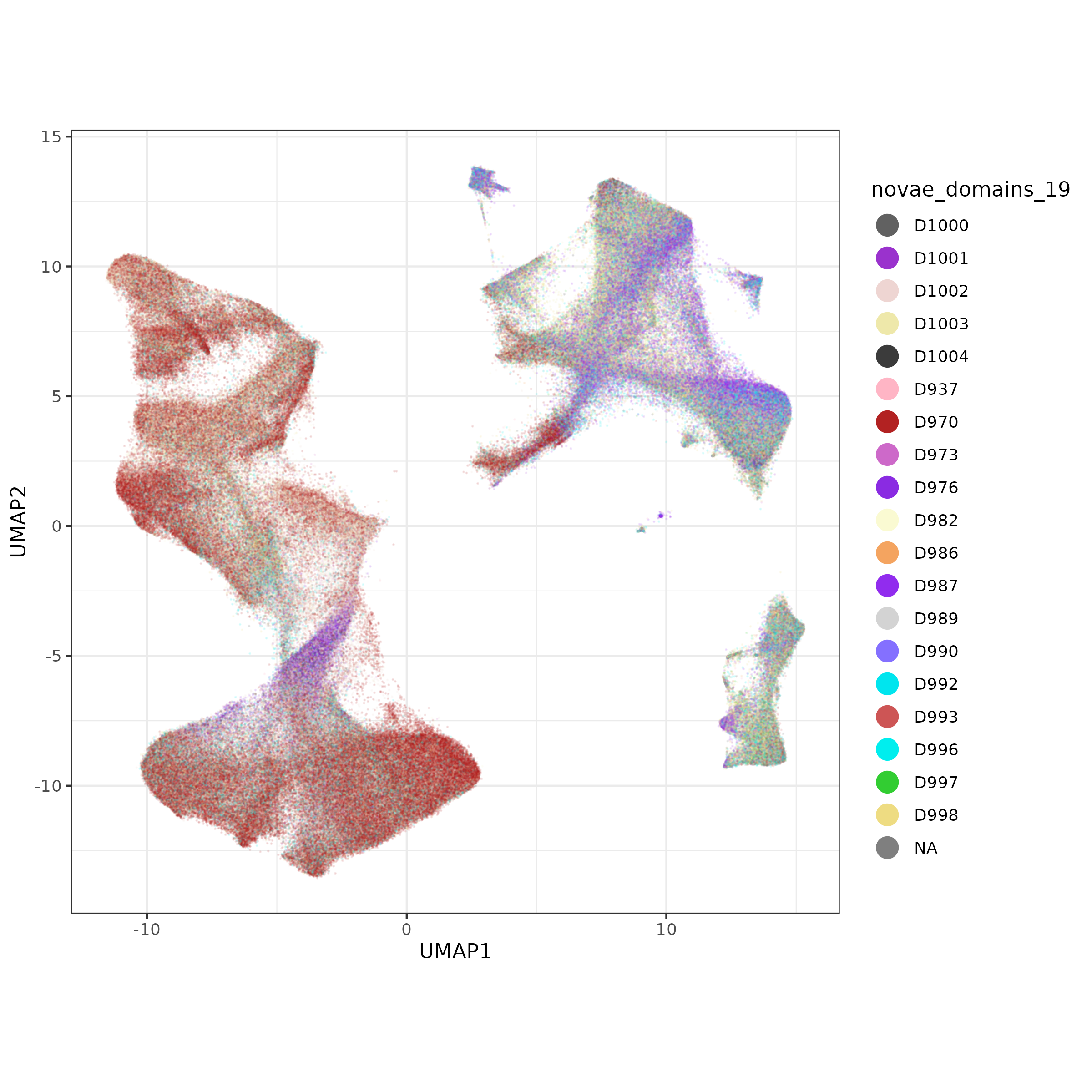
We evaluated domains of various sizes, cutting off the hierarchy at levels leading up to at most 19 distinct domains. For this we visualize the spatial and umap positioning of each hierarchy level.

Domains: 1

Domains: 2

Domains: 3

Domains: 4

Domains: 5

Domains: 6

Domains: 7

Domains: 8

Domains: 9

Domains: 10

Domains: 11

Domains: 12

Domains: 13

Domains: 14

Domains: 15

Domains: 16

Domains: 17

Domains: 18

Domains: 19

Domains: 20

After reviewing the distribution of domains, we decide to focus on the model version with 9 domains. Here are the 9 domains shown separately:

Domain: 1003

Domain: 1007

Domain: 1008

Domain: 1011

Domain: 1012

Domain: 1013

Domain: 1014

Domain: 976

Domain: 987

Based on spatial distribution and minor cell type composition, we assign each domain as a tumor core (TC) domain, interior stroma (IS), or exterior stroma (ES).

novae_9 <- readRDS(file = paste0(niche_dir, "/Data/novae_domains_9_assignments.rds"))

novae_9 <- dplyr::recode(
  novae_9,
  "D987" = "ES1",
  "D1003" = "ES2",
  "D1012" = "TC1",
  "D1013" = "TC2",
  "D976" = "TC3",
  "D1007" = "IS1",
  "D1008" = "IS2",
  "D1014" = "IS3",
  "D1011" = "IS4"
)

saveRDS(novae_9, file = paste0(niche_dir, "/Data/novae_domains_9_namedAssignments.rds"))

3.1 Publication Quality Plots

In this final section we include the code to make high quality plots that appear in the manuscript.

Plot spatially with the novae domain names.

if (!("seu.obj" %in% ls())){
  seu.obj <- readRDS(results_list$seurat_file_postCellTyping)
}

# Read in named novae domains
novae_9 <- readRDS(paste0(niche_dir, "/Data/novae_domains_9_namedAssignments.rds"))

# Extract metadata and add novae domains
df <- seu.obj@meta.data
df$novae_9 <- novae_9[df$cell_ID]

# Manually set named domain colors
domain_colors_9_named <- list(
  TC1 = "#1F77B4",  # Strong blue 
  IS3 = "#FF7F0E",  # Orange
  ES1  = "#2CA02C",  # Green
  IS4 = "#D62728",  # Red
  IS2 = "#9467BD",  # Purple
  ES2 = "#8C564B",  # Brown
  IS1 = "#E377C2",  # Pink
  TC2 = "#7F7F7F",  # Gray
  TC3  = "#17BECF"   # Cyan
)


results_list[['novae_model_1_domain_names9_named']] <- names(domain_colors_9_named)
results_list[['novae_model_1_domain_colors9_named']] <- as.character(domain_colors_9_named)
saveRDS(results_list, results_list_file)

# Set domain order
df$novae_9 <- factor(df$novae_9,
                     levels = sort(unique(as.character(df$novae_9))))


p <- ggplot(data=df %>% filter(!is.na(novae_9)), 
            aes(x=x_slide_mm, y=y_slide_mm, color=novae_9)) + 
  geom_point(size=0.01, alpha=0.6) + 
  theme_void() + 
  coord_fixed() + 
  scale_color_manual(values = domain_colors_9_named, name = "Novae domains") +
  guides(color = guide_legend(override.aes = list(size = 10, alpha=1))) +
  theme(legend.position = c(0,1),
        legend.justification = c(0, 1),
        legend.text=element_text(size=15),
        legend.title = element_text(size = 20))

ggsave(filename = file.path(niche_dir, "Plots", paste0("xy_model_1_domain_9_colorsSelected_named.png")), p,
       width=8, height=14)

# Make a faceted plot showing one domain at a time
# Make a copy of metadata that lacks the cell type
df2 <- dplyr::select(df, -novae_9)

# Sample 5% of cells for background
set.seed(2025)
df2 <- df2[sample(1:nrow(df2), nrow(df2)/20),]

## Plot it
ggplot(df %>% filter(!is.na(novae_9)),
       aes(x = x_slide_mm, y = y_slide_mm)) +
  geom_point(data = df2, color = "grey90", size = 0.01, alpha = 0.05) + # Background cells
  geom_point(color = "black", size = 0.01, alpha = 0.1)+ # Foreground highlighted cells
  coord_fixed() +
  theme_void() +
  facet_wrap(~novae_9) +
  theme(strip.text = element_text(size = 15))

ggsave(paste0(niche_dir, "/Plots/gallery_novae9_positions.png"),
       width = 8, height = 16, units = "in")


# Plot two zoomed regions with polygons
zooms = results_list$zoom_regions

# Read in polygons
polygons <- fread(paste0(objects_dir, "/FlatFiles/flatFiles/BreastCancer/BreastCancer-polygons.csv.gz"))
polygons$x_slide_mm <- polygons$x_global_px * 0.12028/1000
polygons$y_slide_mm <- polygons$y_global_px * 0.12028/1000

# Merge in novae domain
polygons <- merge(polygons, df[,c("cell_ID", "novae_9")], by.x = "cell", by.y = "cell_ID", all.y = T)

# Plot for each zoom region
for (zoom in zooms){
  
  
  idx <- which(
    polygons$x_slide_mm > zoom$xmin &
      polygons$x_slide_mm < zoom$xmax &
      polygons$y_slide_mm > zoom$ymin &
      polygons$y_slide_mm < zoom$ymax
  )
  
  scale_bar <- make_scale_bar_r(polygons[idx, c("x_slide_mm")], polygons[idx, "y_slide_mm"])
  
  ggplot(polygons[idx,],
         aes(x_slide_mm, y_slide_mm, group = cell)) +
    geom_polygon(aes(x_slide_mm, y_slide_mm, group = cell, fill = novae_9)) +
    scale_fill_manual(values = domain_colors_9_named) +
    theme_void() +  
    coord_fixed() +  
    theme(legend.position = "none") +
    scale_bar$bg + 
    scale_bar$rect + 
    scale_bar$label
  ggsave(paste0(niche_dir, "/Plots/", "xy_model_1_domain_9_colorsSelected_named_zoomed_", zoom$region, ".png"),
         width = 4, height = 4, units = "in", dpi = 400)
}

High quality spatial plot of domains and two zoomed regions.

Full tissue

knitr::include_graphics(file.path(niche_dir, "Plots", paste0("xy_model_1_domain_9_colorsSelected_named.png")))

Zoom region 1

knitr::include_graphics(paste0(niche_dir, "/Plots/", 
                               "xy_model_1_domain_9_colorsSelected_named_zoomed_", 
                               "i", ".png"))

Zoom region 2

knitr::include_graphics(paste0(niche_dir, "/Plots/", 
                               "xy_model_1_domain_9_colorsSelected_named_zoomed_", 
                               "ii", ".png"))

Gallery of nine domains in space:

knitr::include_graphics(paste0(niche_dir, "/Plots/gallery_novae9_positions.png"))

Plot the major and minor cell types per domain

if (!("seu.obj" %in% ls())){
  seu.obj <- readRDS(results_list$seurat_file_postCellTyping)
}

# Read in named novae domains
novae_9 <- readRDS(paste0(niche_dir, "/Data/novae_domains_9_namedAssignments.rds"))

# Extract metadata and add novae domains
df <- seu.obj@meta.data
df$novae_9 <- novae_9[df$cell_ID]

# Set minor cell types as an ordered factor
df$minor_cell_type <- factor(df$minor_cell_type,
                             levels = names(results_list$minor_cell_type_color_pal_manual))

# Set domains as ordered factor
df$novae_9 <- factor(df$novae_9,
                     levels = c(
                       "ES1",
                       "ES2",
                       "IS1",
                       "IS2",
                       "IS3",
                       "IS4",
                       "TC1",
                       "TC2",
                       "TC3"
                     ))

# Exclude the few cells not assigned a domain
df <- df %>% filter(!is.na(novae_9))

# Plot it
p <- ggplot(data=df, 
            aes(fill=minor_cell_type, x=novae_9)) + 
  geom_bar(position = "fill") + 
  theme_classic() + 
  scale_fill_manual(values = results_list$minor_cell_type_color_pal_manual, name = "Minor cell type") +
  xlab("Domain") +
  ylab("Fraction of cells in domain") +
  coord_flip() +
  theme(legend.position = "none")

ggsave(filename = file.path(niche_dir, "Plots", paste0("barplot_minorCellTypes_perDomain9_horizontalFormatted.png")), p,
       width=6, height=3)

Distribution of minor cell types across domains:

knitr::include_graphics(file.path(niche_dir, "Plots", paste0("barplot_minorCellTypes_perDomain9.png")))

Plot top pathways per domain, using HieraType marker heatmap code.

# Read in pathway scores
pwd <- readRDS(file = paste0(pathway_dir, "/Data/cellsAUC_full.rds"))

if (!("seu.obj" %in% ls())){
  seu.obj <- readRDS(results_list$seurat_file_postCellTyping)
}

# Read in named novae domains
novae_9 <- readRDS(paste0(niche_dir, "/Data/novae_domains_9_namedAssignments.rds"))

# Extract metadata and add novae domains
df <- seu.obj@meta.data
df$novae_domain_9 <- novae_9[df$cell_ID]
if(all(df$cell_ID) == colnames(pwd)){
  
  ## Heatmap of pathways by domain
  pwfctbl <- 
    HieraType::clusterwise_foldchange_metrics(normed = pwd
                                              ,metadata = df[,c("novae_domain_9", "cell_ID")]
                                              ,cluster_column = "novae_domain_9")
  
  
  # Save it
  saveRDS(pwfctbl, file = paste0(niche_dir, "/Data/pwfctbl_novae9.rds"))
  
  # Remove NA cluster and 'reactome' from pathway names
  pwfctbl <- pwfctbl[!(is.na(pwfctbl$cluster)),]
  pwfctbl$gene <- gsub("REACTOME-", "", pwfctbl$gene)
  
  # Replace some pathway names with shorter abbreviations for better plotting
  pwfctbl$gene <- dplyr::recode(pwfctbl$gene,
                                "TP53-REGULATES-TRANSCRIPTION-OF-SEVERAL-ADDITIONAL-CELL-DEATH-GENES-WHOSE-SPECIFIC-ROLES-IN-P53-DEPENDENT-APOPTOSIS-REMAIN-UNCERTAIN" = "(*)TP53-REGULATED-CELL-DEATH",
                                "CROSS-PRESENTATION-OF-PARTICULATE-EXOGENOUS-ANTIGENS-PHAGOSOMES" = "(*)EXOGENOUS-ANTIGENS-PRESENTATION",
                                "NR1H2-NR1H3-REGULATE-GENE-EXPRESSION-LINKED-TO-LIPOGENESIS" = "(*)NR1H2-NR1H3-REGULATED-LIPOGENESIS",
                                "DEFECTIVE-CHST14-CAUSES-EDS-MUSCULOCONTRACTURAL-TYPE" = "(*)DEFECTIVE-CHST14-CAUSES-EDS")
  
  # Change pathway names to first letter capitalized
  pwfctbl$gene <- stringr::str_to_sentence(pwfctbl$gene)
  pwfctbl$gene <- gsub("-", " ", pwfctbl$gene)
  
  ## Plot it as a tile plot since fraction of cells doesn't have much meaning for a pathway
  # Extract features to use and order as in HieraType code
  fctable <- data.table::copy(pwfctbl)
  fctable[, `:=`(scaled_fold_change, fold_change/max(fold_change)), 
          by = gene]
  fctable[, `:=`(scaled_expr, cluster_expr/max(cluster_expr)), 
          by = gene]
  fctable[is.na(scaled_fold_change), `:=`(scaled_fold_change, 
                                          0)]
  fctable[is.na(scaled_expr), `:=`(scaled_expr, 0)]
  dmat <- data.table::dcast(fctable, gene ~ cluster, 
                            value.var = "scaled_fold_change")
  fc_mat <- as.matrix(dmat[, -c("gene"), with = FALSE])
  rownames(fc_mat) <- dmat[, gene]
  
  featsuse <- unique(c(fctable[order(-fold_change)][cluster_prop > 
                                                      0.05, head(.SD, 3), by = cluster][, 
                                                                                        unique(gene)]))
  
  suppressMessages(hmap <- ComplexHeatmap::Heatmap(fc_mat[featsuse, 
  ]))
  suppressMessages(grid::grid.grabExpr(hmap <- ComplexHeatmap::draw(hmap)))
  
  gene_order <- featsuse[ComplexHeatmap::row_order(hmap)]
  
  ct_order <- colnames(fc_mat)[ComplexHeatmap::column_order(hmap)]
  
  pd <- fctable[gene %in% featsuse]
  pd[, `:=`(gene, factor(gene, levels = gene_order))]
  pd[, `:=`(cluster, factor(cluster, levels = ct_order))]
  
  
  pd[, `:=`(rnk, rank(-fold_change)), by = gene]
  pd[, `:=`(gene, factor(gene, levels = pd[rnk == 1][order(cluster, 
                                                           -fold_change)][, unique(gene)]))]
  
  
  ggplot(as.data.frame(pd),
         aes(y = cluster, x = gene, fill = scaled_expr)) +
    geom_tile() +
    scale_fill_gradientn(colors = RColorBrewer::brewer.pal(9, "Blues"), 
                         name = "Scaled Pathway Score") +
    theme_classic() +
    theme(axis.text.x = element_text(angle = 90, hjust = 1, vjust = 0.5, 
                                     size = 12),
          axis.title.x = element_blank(),
          axis.text.y = element_text(size = 12),
          axis.title.y = element_blank()) +
    coord_flip()
  ggsave(filename = paste0(niche_dir, 
                           "/Plots/heatmap_pathways_by_domain_formatted.png"),
         height = 5, width = 8, units = "in", dpi = 300)
  
  
}

Heatmap of top pathways by domain:

knitr::include_graphics(paste0(niche_dir, "/Plots/heatmap_pathways_by_domain_formatted.png"))