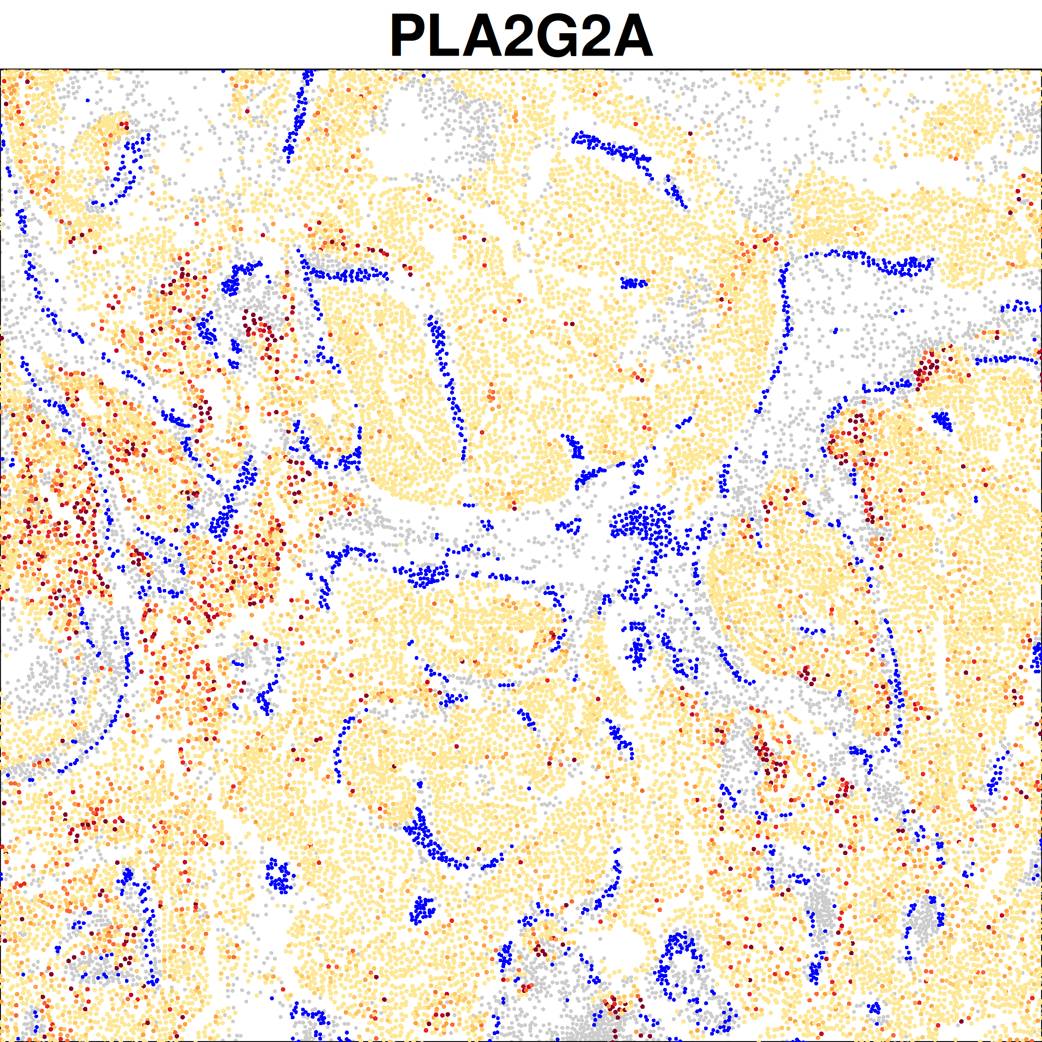
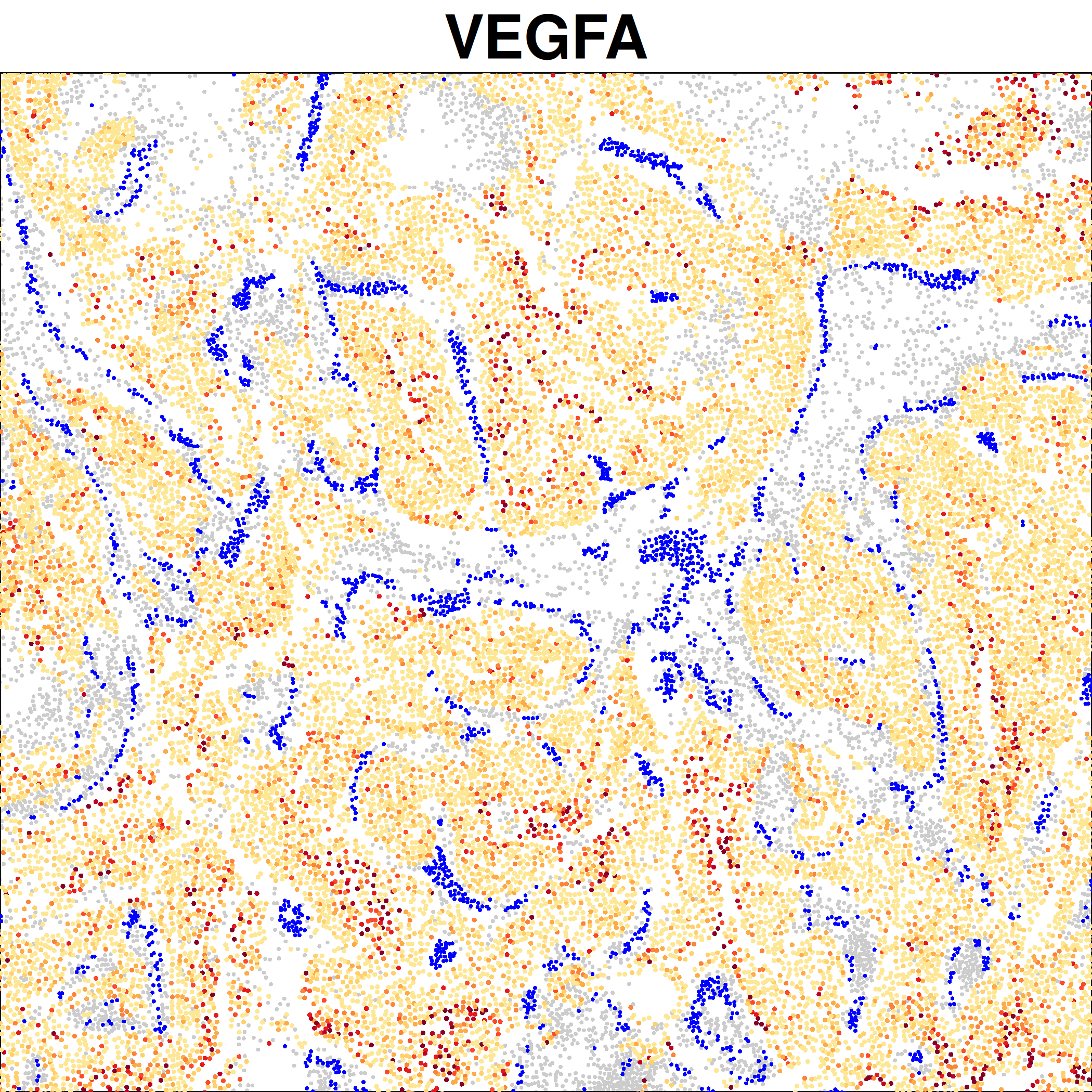
In this section we focus on the vasculature within the tumor. One of the hallmarks of cancer is inducing angiogenesis, so we identify vessels in the tissue and then examine transcriptional changes near the vasculature across tumor subtypes.
6.1 Identify vasculature
We use dbscan to identify vessels as groups of co-localized endothelial cells and pericytes.
Show the code
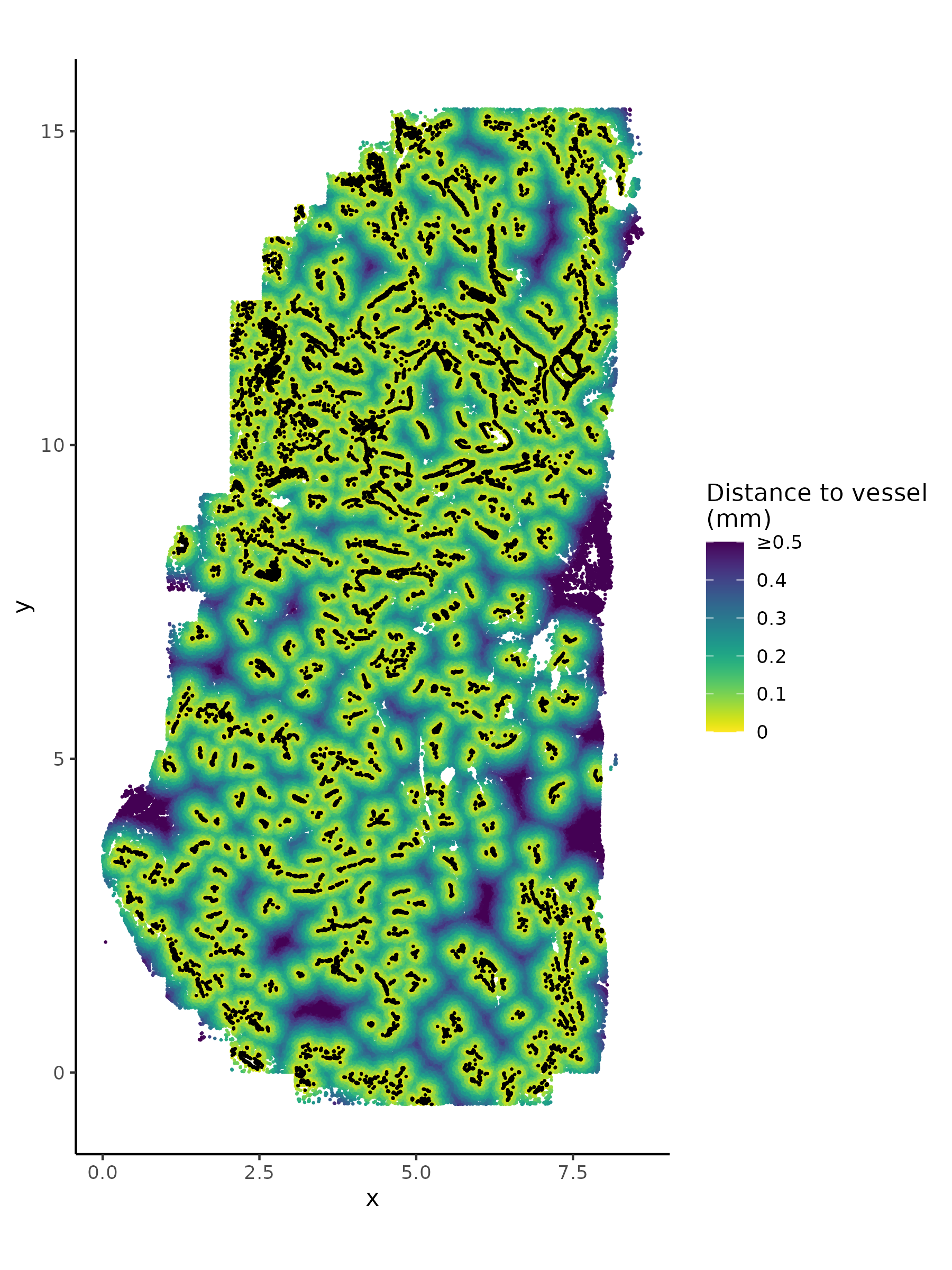
# if there's no seurat object, read it inif (!("seu.obj"%in%ls())){ seu.obj <-readRDS(results_list$seurat_file_postCellTyping)}# Extract spatial locationsxy <-data.frame("x"= seu.obj@meta.data$x_slide_mm, "y"= seu.obj@meta.data$y_slide_mm)rownames(xy) <-rownames(seu.obj@meta.data)# identify vessels:sub <- seu.obj@meta.data$major_cell_type =="Vasculature"db <- dbscan::dbscan(xy[sub, ], eps =0.1, minPts =20)sub2 <-which(sub)[db$cluster >0]# distance to nearest vessel:dist2vessel <- FNN::get.knnx(data = xy[sub2, ], # 2-column matrix of xy locationsquery = xy, k =1)$nn.distsaveRDS(dist2vessel, file =paste0(vessel_dir, "/Data/dist2vessel.rds"))saveRDS(sub2, file =paste0(vessel_dir, "/Data/cells_in_vessels.rds"))# Plot vessels plus distance to nearest vesselplot.df <- xyplot.df$dist_to_vessel <- dist2vessel[,1]ggplot(plot.df, aes(x = x, y = y, color = dist_to_vessel)) +geom_point(size =0.1) +scale_color_viridis(direction =-1, limits =c(0, 0.5), oob = scales::squish,labels =c("0", "0.1", "0.2", "0.3", "0.4", "≥0.5"),name ="Distance to vessel\n(mm)") +geom_point(data = plot.df %>%filter(dist_to_vessel ==0),aes(x = x, y = y), color ="black", size =0.1) +coord_fixed() +theme_classic()ggsave(filename =paste0(vessel_dir, "/Plots/XY_distanceToVessel_plusVessels.png"),width =6, height =8, units ="in", dpi =300)
Plot of vessels and distance to nearest vessel in space:
6.2 Differential expression by vasculature distance
We run DE on each tumor subtype by proximity to vessels to ask what genes are up or downregulated in tumor cells near the vessels. This could indicate genes that are inducing angiogenesis (near vessels) or indicators of hypoxia (far from vessels).
Show the code
# if there's no seurat object, read it inif (!("seu.obj"%in%ls())){ seu.obj <-readRDS(results_list$seurat_file_postCellTyping)}# Add distance to nearest vesseldist2vessel <-readRDS(file =paste0(vessel_dir, "/Data/dist2vessel.rds"))seu.obj@meta.data$dist2vessel <- dist2vessel### Add a normalized expression matrixseu.obj@meta.data$totalcounts <- seu.obj@meta.data$nCount_RNAtotalcount_scalefactors <-mean(seu.obj@meta.data[["totalcounts"]]) / seu.obj@meta.data[["totalcounts"]]names(totalcount_scalefactors) <- seu.obj@meta.data[["cell_ID"]]seu.obj <- Seurat::SetAssayData(seu.obj ,"data" ,seu.obj[["RNA"]]@counts %*% Matrix::Diagonal(x=totalcount_scalefactors, names=colnames(seu.obj)) )# Calculate overlap metricoverlap_metrics <-smiDE::contamination_ratio_metric(assay_matrix = seu.obj[["RNA"]]@data ,metadata = seu.obj@meta.data ,cellid_col ="cell_ID" ,cluster_col ="minor_cell_type" ,sdimx_col ="x_slide_mm" ,sdimy_col ="y_slide_mm" ,radius =0.05 )saveRDS(overlap_metrics, file =paste0(vessel_dir, "/Data/overlap_metrics.rds"))# Calculate shared pre-de objpre_de_obj <-pre_de(metadata = seu.obj@meta.data ,cell_type_metadata_colname ="minor_cell_type" ,mm_radius =0.05 ,sdimx_colname ="x_slide_mm" ,sdimy_colname ="y_slide_mm" ,verbose=TRUE ,adjacencies_only=TRUE)saveRDS(pre_de_obj, file =paste0(vessel_dir, "/Data/pre_de_obj.rds"))# Run DE for each tumor typetumor_types <- seu.obj@meta.data %>%filter(major_cell_type =="Tumor") %>%pull(minor_cell_type) %>%unique()for(ct in tumor_types){# Consider only genes higher in the cell type of interest than other surrounding cell types genes_to_analyze <- overlap_metrics[minor_cell_type==ct][ratio <1][["target"]]# Run de de_obj <-smi_de(assay_matrix = seu.obj[["RNA"]]@counts[genes_to_analyze,] ,metadata = seu.obj@meta.data[which(seu.obj@meta.data$minor_cell_type == ct),] ,formula =~RankNorm(otherct_expr) + dist2vessel +offset(log(totalcounts)) ,pre_de_obj = pre_de_obj ,neighbor_expr_cell_type_metadata_colname ="minor_cell_type" ,neighbor_expr_totalcount_normalize =TRUE ,neighbor_expr_totalcount_scalefactor = totalcount_scalefactors ,family="nbinom2" ,targets=genes_to_analyze ,groupVar ="dist2vessel" ,nCores=12 )saveRDS(de_obj, file =paste0(vessel_dir, "/Data/de_obj_vesselDist_", gsub("\\+", "", gsub(" ", "_", ct)), ".rds"))}
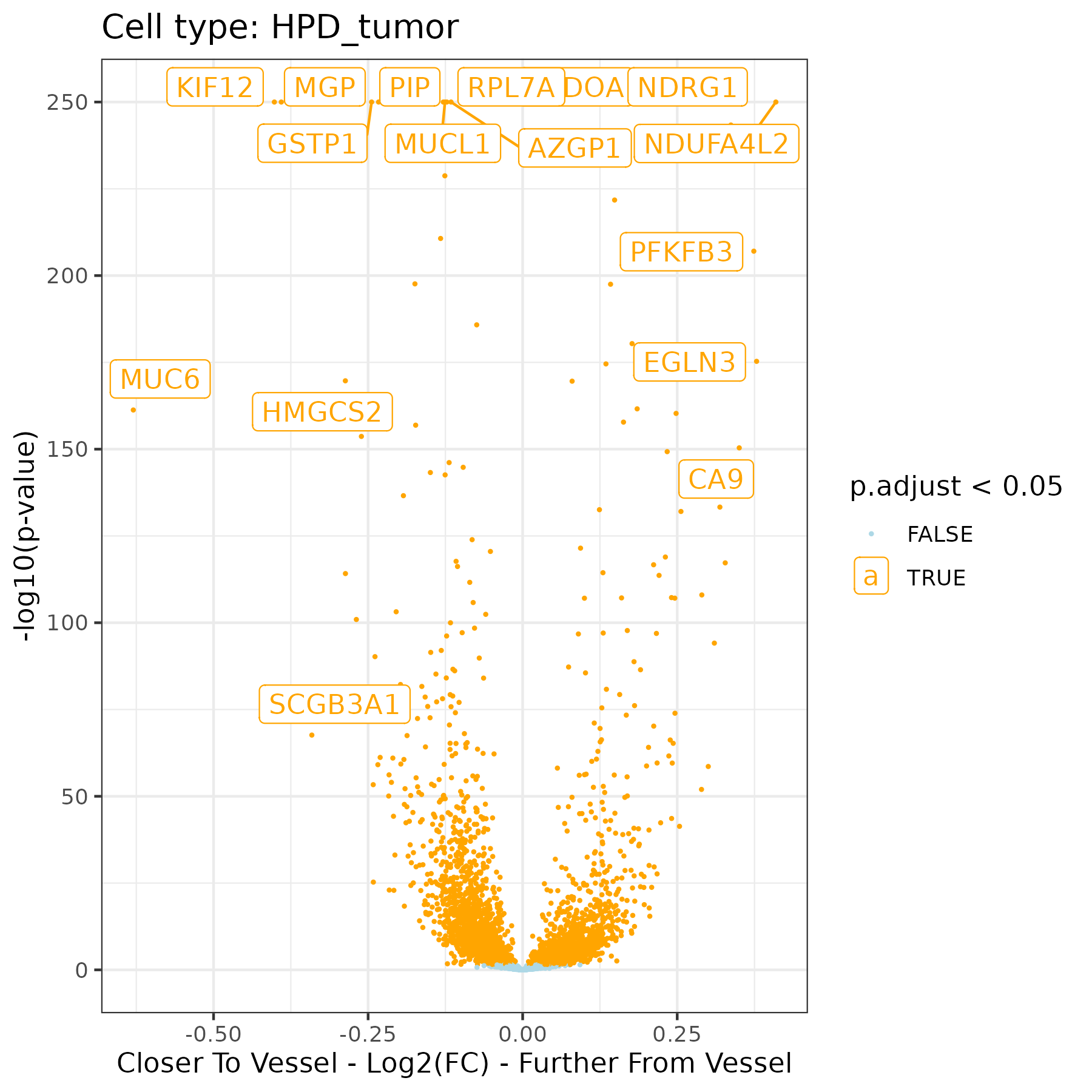
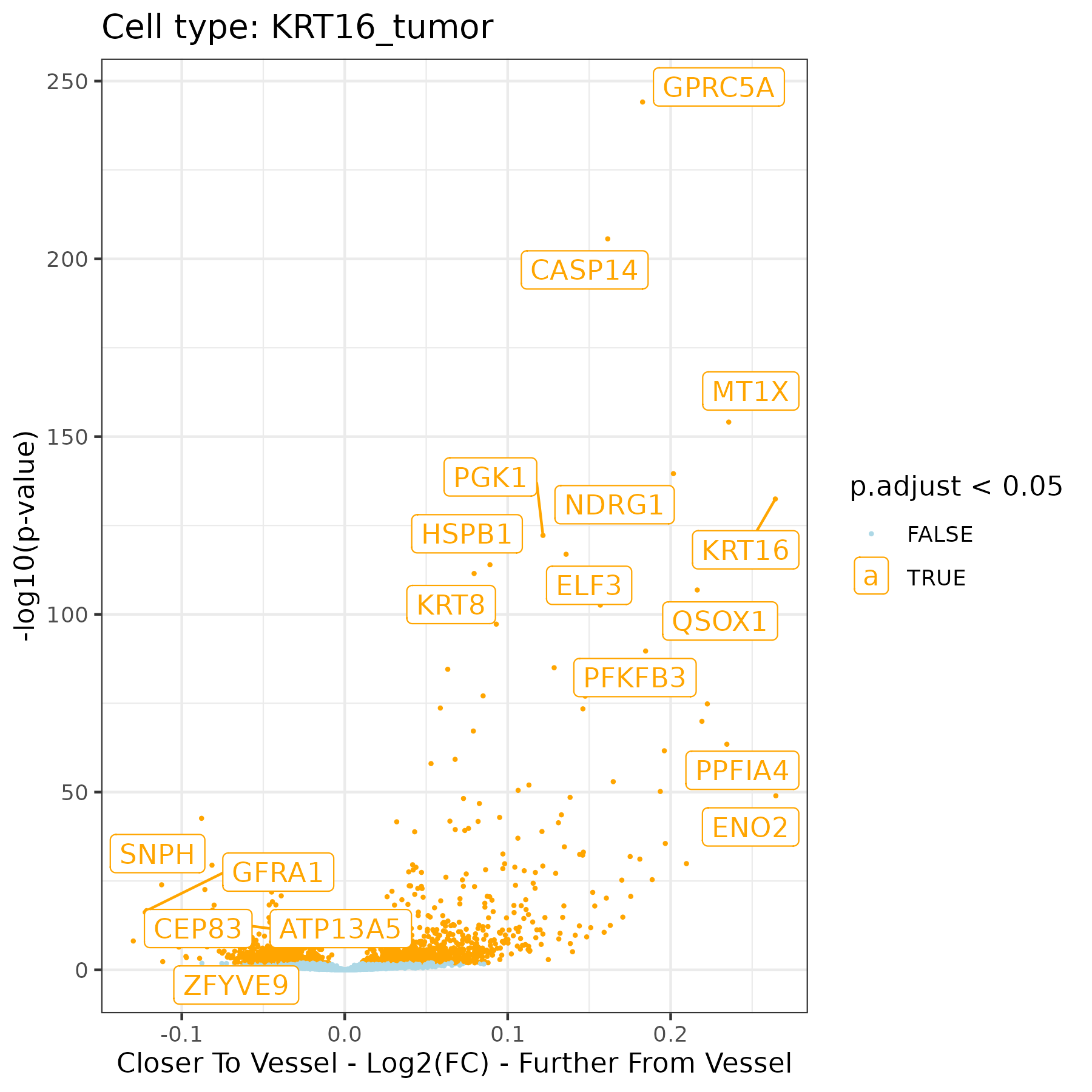
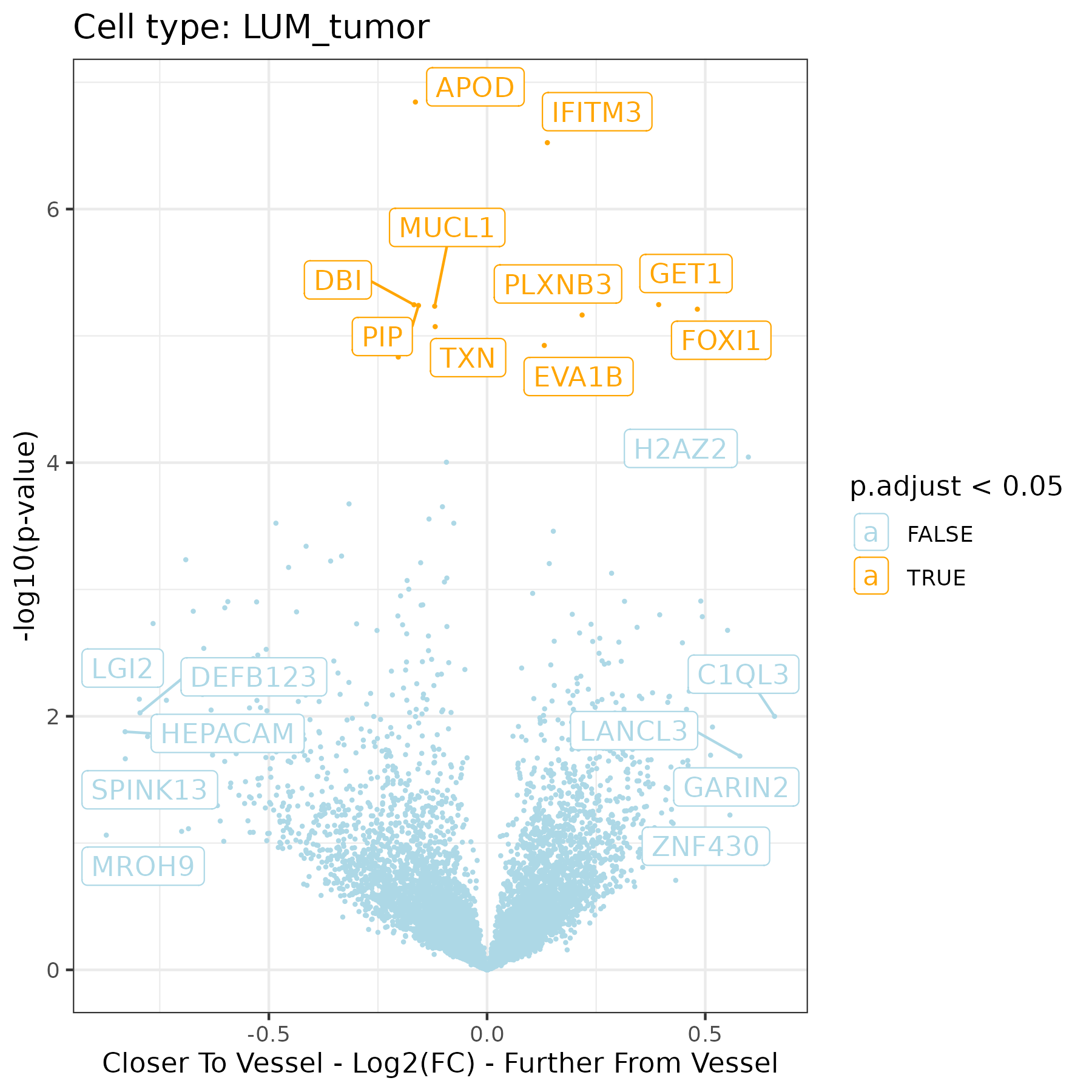
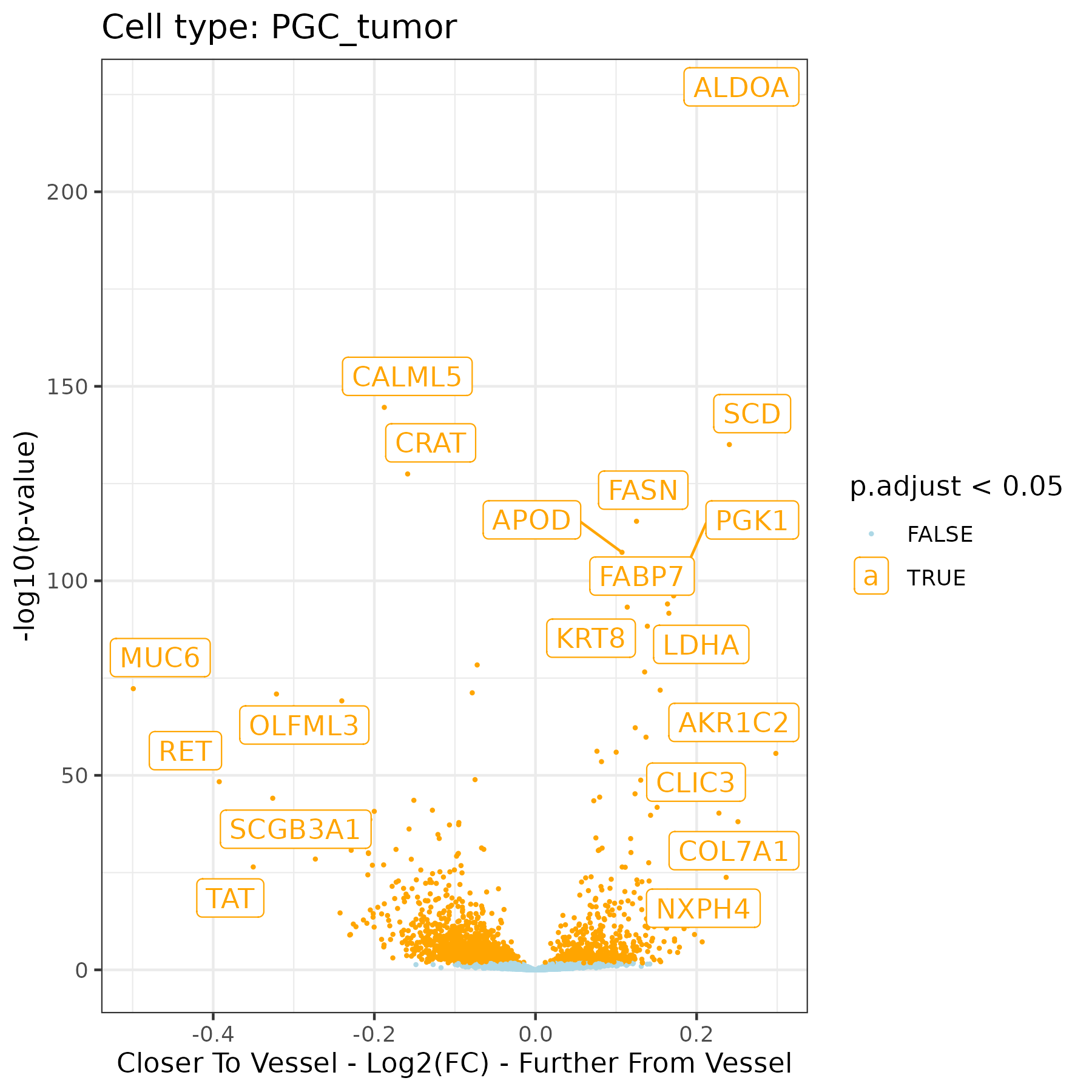
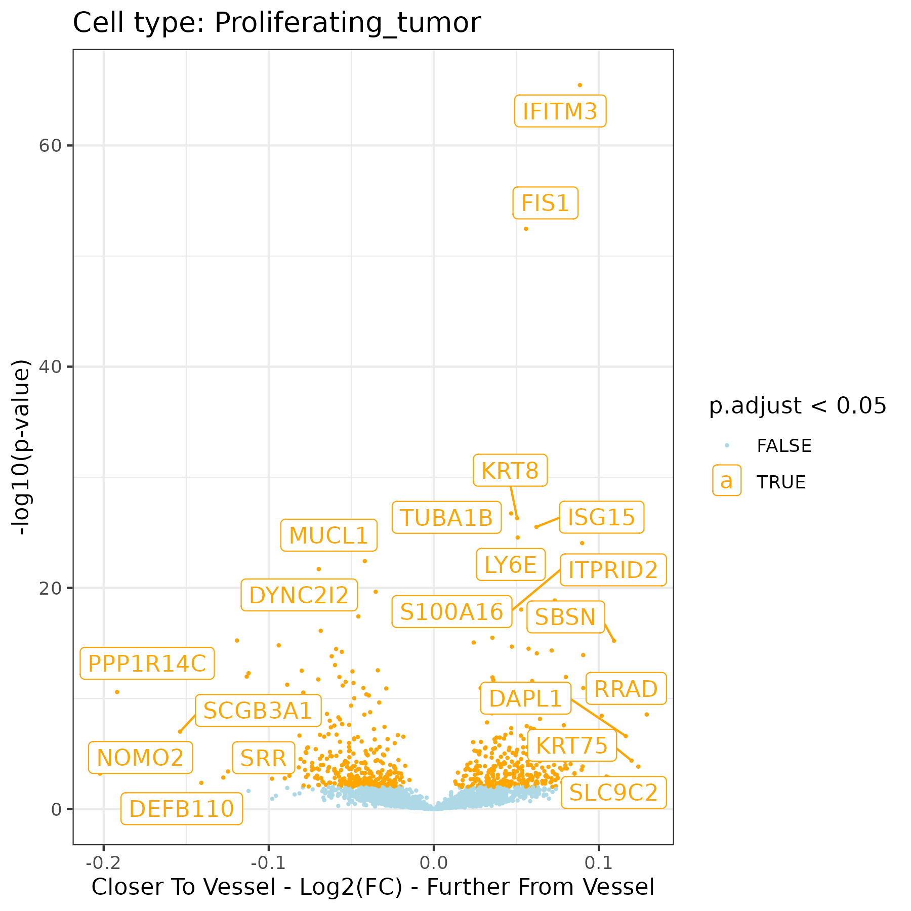
Plot DE results with a volcano showing genes as a comparison between mean distance to a vessel and one SD away, for each tumor subtype. Label the genes with most extreme fold changes and / or p-values.
Show the code
# List DE file namesde_files <-dir(paste0(vessel_dir, "/Data"), pattern ="de_obj_vesselDist")# Make a plot for each de filefor (de_file in de_files){# Read in results de_res <-readRDS(paste0(vessel_dir, "/Data/", de_file))# Extract cell type ct <-gsub("de_obj_vesselDist_", "", gsub(".rds", "", de_file))# Extract pairwise de_res <-results(de_res)$pairwise# Extract contrast of interest de_res <- de_res %>%filter(term =="dist2vessel")# Add adjusted p de_res$p.adjust <-p.adjust(de_res$p.value, method ="BH")# Select targets to label smallest_ratio <- de_res %>%arrange(ratio) %>%slice_head(n =5) largest_ratio <- de_res %>%arrange(desc(ratio)) %>%slice_head(n =5) smallest_p_adjust <- de_res %>%arrange(p.adjust) %>%slice_head(n =10) targets_to_label <-unique(c(smallest_ratio$target, largest_ratio$target, smallest_p_adjust$target))# Plot itggplot(de_res, aes(x =log2(ratio), y =-log10(p.value+10^-250), color = p.adjust <0.05)) +geom_point(size =0.3) +scale_color_manual(values =c("lightblue", "orange")) +geom_label_repel(data = de_res %>%filter(target %in% targets_to_label),aes(x =log2(ratio), y =-log10(p.value+10^-250), color = p.adjust <0.05,label = target)) +theme_bw() +xlab("Closer To Vessel - Log2(FC) - Further From Vessel") +ylab("-log10(p-value)") +ggtitle(paste0("Cell type: ", ct))ggsave(paste0(vessel_dir, "/Plots/volcano_dist2vessel_ct_", ct, ".png"),width =6, height =6, units ="in")}
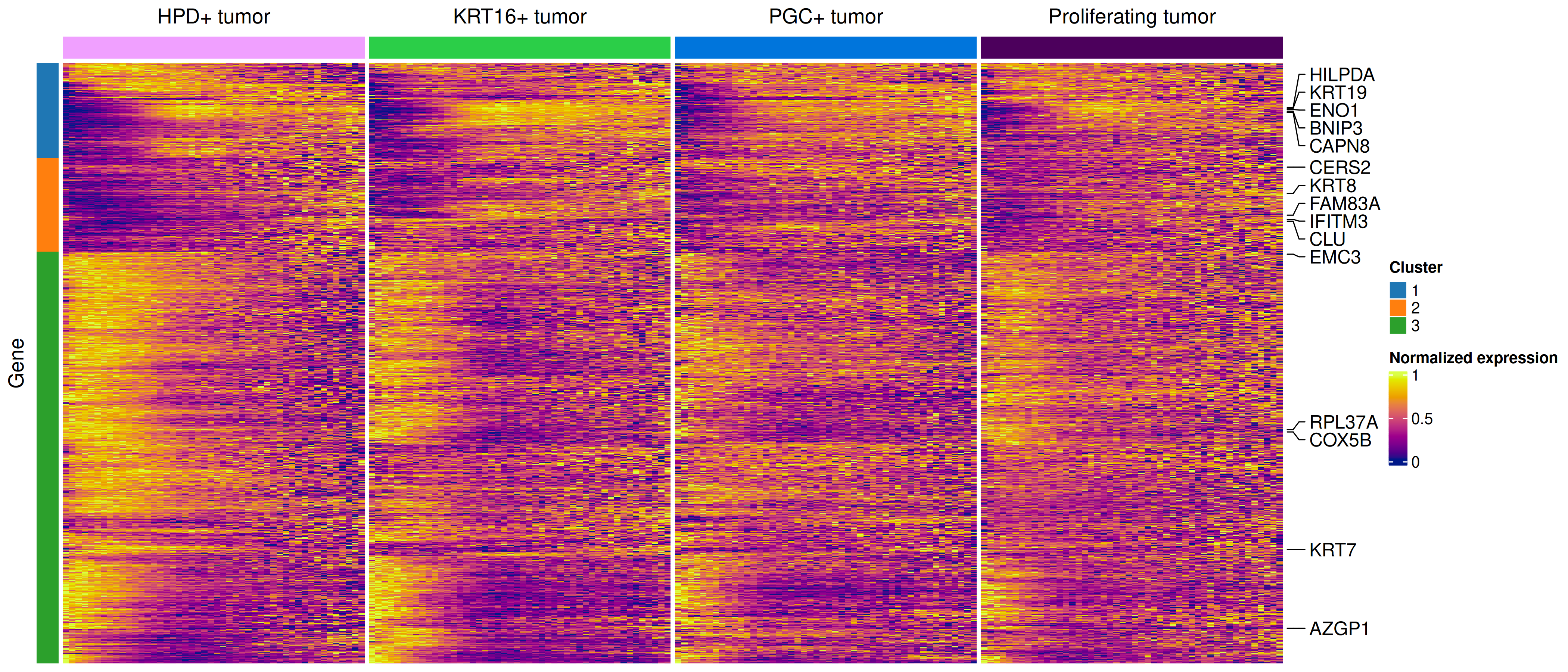
Plot the top DE genes by tumor type as a heatmap with x-axis binned distance to vessel and y axis gene, normalized to max expression. Make one long heatmap with small gaps between each cell type but genes aligned. Also save a table of DE results to provide as a supplementary table.
Show the code
# if there's no seurat object, read it inif (!("seu.obj"%in%ls())){ seu.obj <-readRDS(results_list$seurat_file_postCellTyping)}# Add distance to nearest vesseldist2vessel <-readRDS(file =paste0(vessel_dir, "/Data/dist2vessel.rds"))seu.obj@meta.data$dist2vessel <- dist2vessel# Bin distances with 90% of max as top distancemetadata <- seu.obj@meta.datametadata$dist2vessel_2 <-ifelse(metadata$dist2vessel <quantile(dist2vessel, 0.9), metadata$dist2vessel, NA)metadata <- metadata %>%mutate(distance_bin =cut(dist2vessel_2, breaks =50))# Generate a normalized expression matrixseu.obj@meta.data$totalcounts <- seu.obj@meta.data$nCount_RNAtotalcount_scalefactors <-mean(seu.obj@meta.data[["totalcounts"]]) / seu.obj@meta.data[["totalcounts"]]names(totalcount_scalefactors) <- seu.obj@meta.data[["cell_ID"]]norm_mtx <- seu.obj[["RNA"]]@counts %*% Matrix::Diagonal(x=totalcount_scalefactors, names=colnames(seu.obj))# List DE file namesde_files <-dir(paste0(vessel_dir, "/Data"), pattern ="de_obj_vesselDist")# Gather DE results to select genesde_results_list <-lapply(de_files, function(de_file) { de_res <-readRDS(file.path(vessel_dir, "Data", de_file)) df <-results(de_res)$pairwise[, c("target", "p.value", "ratio", "term")] df <- df %>%filter(term =="dist2vessel") df$p.adjust <-p.adjust(df$p.value, method ="fdr") df$cell_type <-gsub("de_obj_vesselDist_", "", gsub(".rds", "", de_file))colnames(df) <-c("gene", "p_value", "ratio", "term", "p.adjust", "cell_type")return(df)})# Combine all data frames into onede_results_combined <-do.call(rbind, de_results_list)# Save DE results to a table to be included as supplementary information.write.csv(as.data.frame(de_results_combined),file =paste0(vessel_dir, "/Data/TumorVesselDistanceDE_table.csv"),row.names =FALSE)# Select top 1000 consistently DE genes to plottop_genes <- de_results_combined %>%group_by(gene) %>%filter(n_distinct(cell_type) >=4) %>%# Keep genes evaluated in ≥ 4 cell typessummarize(mean_p =mean(p.adjust, na.rm =TRUE), .groups ="drop") %>%arrange(mean_p) %>%slice_head(n =1000) %>%pull(gene)# Aggregate expression by gene, distance bin, and cell typeexpr_wide <-matrix(nrow =1000, ncol =0)if(all(colnames(norm_mtx) == metadata$cell_id)){for (ct ingrep("tumor", unique(metadata$minor_cell_type), value =TRUE)){print(ct)for(dist_bin insort(unique(metadata$distance_bin))){ idx <-intersect(which(metadata$minor_cell_type == ct),which(metadata$distance_bin == dist_bin))print(dist_bin)if(length(idx)>100){ # Only calculate means if there are at least 100 cells mean_exp <-rowMeans(norm_mtx[top_genes, intersect(which(metadata$minor_cell_type == ct),which(metadata$distance_bin == dist_bin))]) expr_wide <-cbind(expr_wide, mean_exp)colnames(expr_wide)[ncol(expr_wide)] <-paste0(ct, "_", strsplit(as.character(dist_bin), ",|\\(")[[1]][2]) } } }}# Save the wide expression matrix going into heatmapsaveRDS(expr_wide, file =paste0(vessel_dir, "/Data/top1000_tumorExp_byVesselDist_expr_wide_matrix.rds"))# Remove LUM+ (also known as ITGB6+) as it's disrupting scalingexpr_wide_noLum <- expr_wide[,-grep("LUM", colnames(expr_wide))]# Also remove the first distance bin which is likely impacted by low cell number and / or segmentation overlap with vesselsexpr_wide_noLum <- expr_wide_noLum[,-grep("0.00596", colnames(expr_wide_noLum))]# Normalize within each cell type separately# Initialize result matrixmat <- expr_wide_noLummat_norm <-matrix(NA, nrow =nrow(mat), ncol =ncol(mat))rownames(mat_norm) <-rownames(mat)colnames(mat_norm) <-colnames(mat)# Extract cell types from normed matrixcell_types <-sapply(strsplit(colnames(mat_norm), "_"), `[`, 1)# Normalize within each cell type groupfor (ct inunique(cell_types)) { cols <-which(cell_types == ct) mat_norm[, cols] <-t(apply(mat[, cols, drop =FALSE], 1, function(x) { (x -min(x)) / (max(x) -min(x)) }))}# Create annotation for columns# Follow tumor colors from tumor only plotmy_pal <- pals::alphabet(n =5)my_pal[5] <-alphabet(n=7)[7]my_pal[3] <-alphabet(n=25)[15]names(my_pal) <-grep("tumor", unique(seu.obj$minor_cell_type), value = T)my_sample_col_ano <-HeatmapAnnotation(cell_type =cell_types,show_annotation_name =FALSE,col =list(cell_type = my_pal),show_legend =FALSE)# Set up coloring with plasma palettecol_fun = circlize::colorRamp2(range(mat_norm), hcl_palette ="plasma", reverse =FALSE)# Make heatmap to extract gene clusters and get pathways enrichedhm <-draw(ComplexHeatmap::Heatmap(mat_norm, # Remove name from fill legendname ="Normalized expression",# Keep original col ordercolumn_order =colnames(mat_norm),# Add top annotation (legend with cell type) top_annotation = my_sample_col_ano,# ACTUAL SPLIT by cell typecolumn_split = cell_types,show_row_names =FALSE, show_column_names =FALSE,show_row_dend =FALSE, show_column_dend =FALSE,row_title =NULL,col = col_fun))# Extract dendrogramrow_dend <-row_dend(hm)# Cut the dendrogram into 3 clustersclusters <-cutree(as.hclust(row_dend), k =3)# Make a row annotation for these clusters# Define colors for each clustercluster_colors <-structure(c("#1f77b4", "#ff7f0e", "#2ca02c"), # blue, orange, greennames =as.character(sort(unique(clusters))))# Create a row annotation for clusterscluster_anno <-rowAnnotation(Cluster = clusters,col =list(Cluster = cluster_colors),show_annotation_name =FALSE)# Get five genes from each clustergene_df <-as.data.frame(mat_norm)gene_df$cluster <- clusters# Calculate row variancegene_df$variance <-apply(mat_norm, 1, var)# Get top 5 genes by variance in each clustertop_cluster_genes <- gene_df %>%mutate(gene =rownames(gene_df)) %>%group_by(cluster) %>%top_n(5, variance) %>%arrange(cluster, desc(variance)) %>% dplyr::select(gene)# Get corresponding rowstop_cluster_gene_rows <-which(row.names(mat_norm) %in% top_cluster_genes$gene)# Set up annotation with genes to highlight, selected across 3 gene clusters# Many of these are relevant to vasculature / angiogenesis / inflammationha =rowAnnotation(foo =anno_mark(at = top_cluster_gene_rows, labels =rownames(mat_norm)[top_cluster_gene_rows]))# Plot heatmappng(filename =paste0(vessel_dir, "/Plots/heatmap_DEGs_byVesselDist_allTumorTypesExceptLUM_oneHM_clusterGenesPathways.png"),width =14, height =6, units ="in", res =300)ComplexHeatmap::Heatmap(mat_norm, # Remove name from fill legendname ="Normalized expression",# Keep original col ordercolumn_order =colnames(mat_norm),# Add top annotation (legend with cell type) top_annotation = my_sample_col_ano,# ACTUAL SPLIT by cell typecolumn_split = cell_types,show_row_names =FALSE, show_column_names =FALSE,show_row_dend =FALSE, show_column_dend =FALSE,row_title ="Gene",#column_title = "Distance to vessel",#column_title_side = "bottom",col = col_fun,right_annotation = ha,left_annotation = cluster_anno)dev.off()# Get top enriched pathways from each clusterreactome_enrich_res <-list()for(geneCluster inunique(gene_df$cluster)){ gene_ids <-bitr(row.names(gene_df)[which(gene_df$cluster == geneCluster)],fromType ="SYMBOL",toType ="ENTREZID",OrgDb = org.Hs.eg.db)# Perform enrichment analysis (unranked list) reactome_enrich <-enrichPathway(gene = gene_ids$ENTREZID,organism ="human",pvalueCutoff =0.05,readable =TRUE) reactome_enrich_res[[geneCluster]] <- reactome_enrich}saveRDS(reactome_enrich_res, file =paste0(vessel_dir, "/Data/reactome_enrich_tumorsVesselCluster_.rds"))
Heatmap showing top 1000 genes across four most prominent tumor subtypes:
reactome_enrich_res <-readRDS(file =paste0(vessel_dir, "/Data/reactome_enrich_tumorsVesselCluster_.rds"))# Define top pathways per clusterpathways <-list()for (i in1:length(reactome_enrich_res)){ pathways[[i]] <- reactome_enrich_res[[i]]@result$Description[1:5]}print(pathways)
[[1]]
[1] "Gluconeogenesis"
[2] "Glycolysis"
[3] "Metabolism of carbohydrates and carbohydrate derivatives"
[4] "Glucose metabolism"
[5] "Differentiation of Keratinocytes in Interfollicular Epidermis in Mammalian Skin"

[[2]]
[1] "Neutrophil degranulation"
[2] "Metabolic disorders of biological oxidation enzymes"
[3] "Apoptotic cleavage of cell adhesion  proteins"
[4] "Regulation of localization of FOXO transcription factors"
[5] "SARS-CoV-2 targets host intracellular signalling and regulatory pathways"

[[3]]
[1] "Regulation of expression of SLITs and ROBOs"
[2] "Nonsense Mediated Decay (NMD) independent of the Exon Junction Complex (EJC)"
[3] "L13a-mediated translational silencing of Ceruloplasmin expression"
[4] "Eukaryotic Translation Initiation"
[5] "Cap-dependent Translation Initiation"
6.3 Plots of selected genes’ trends:
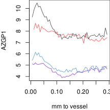
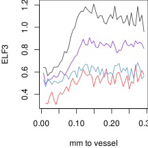
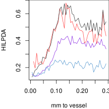
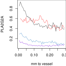
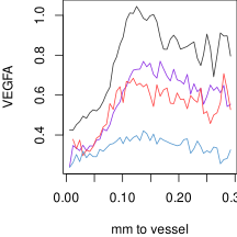
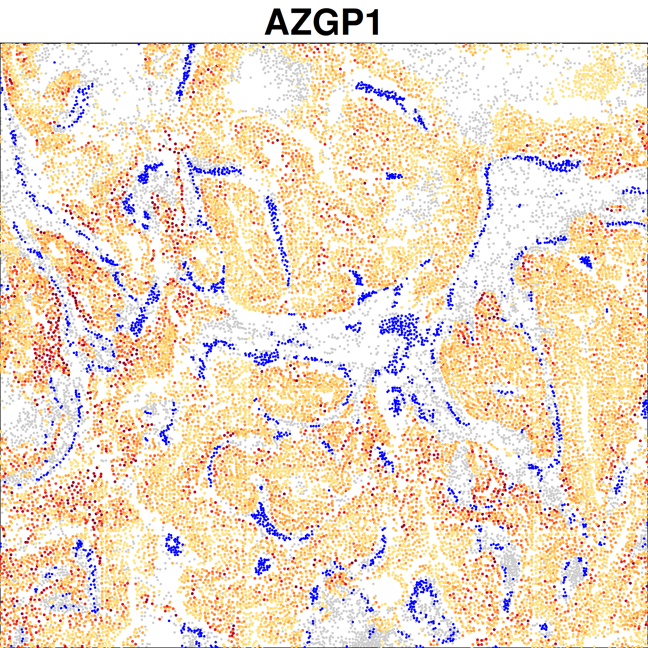
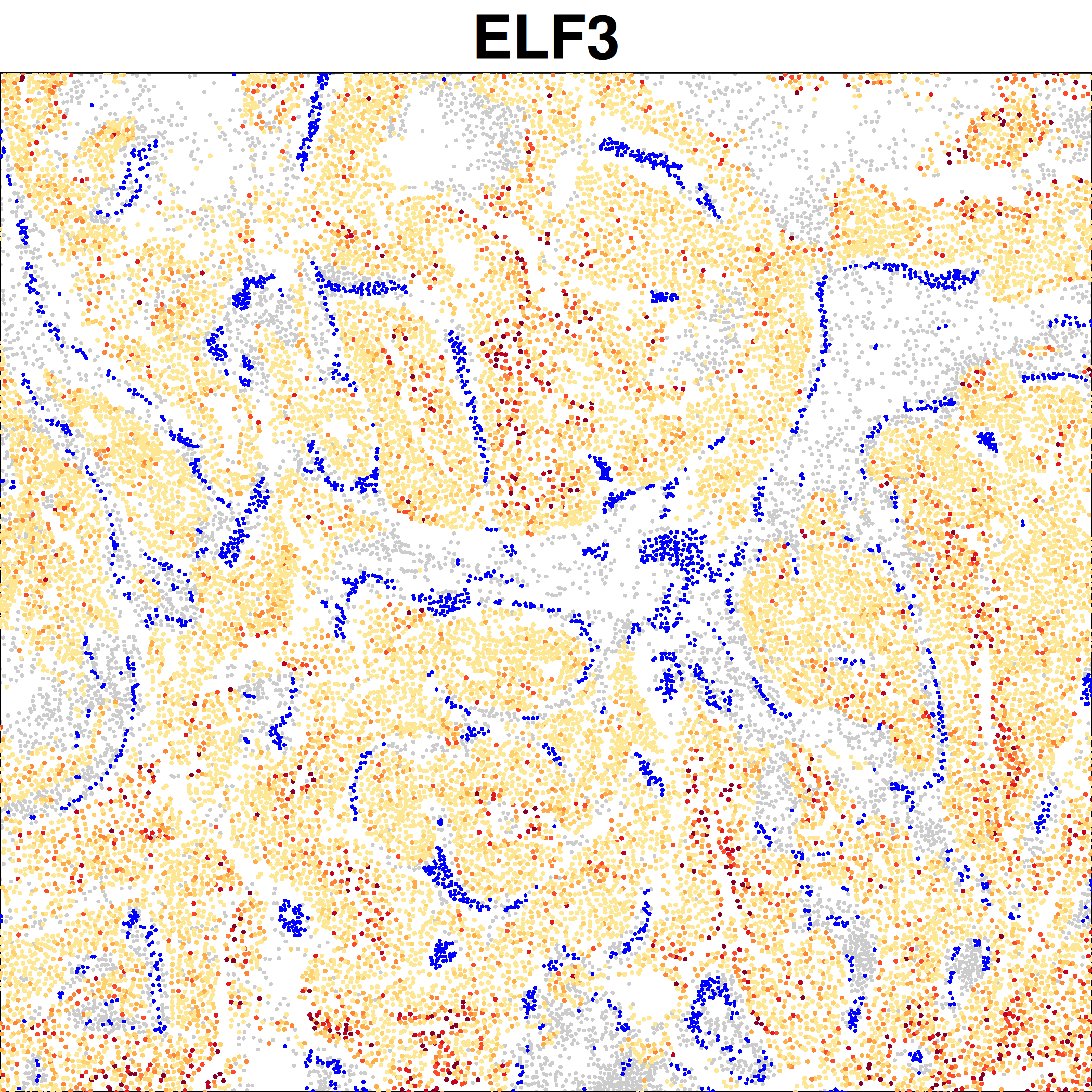
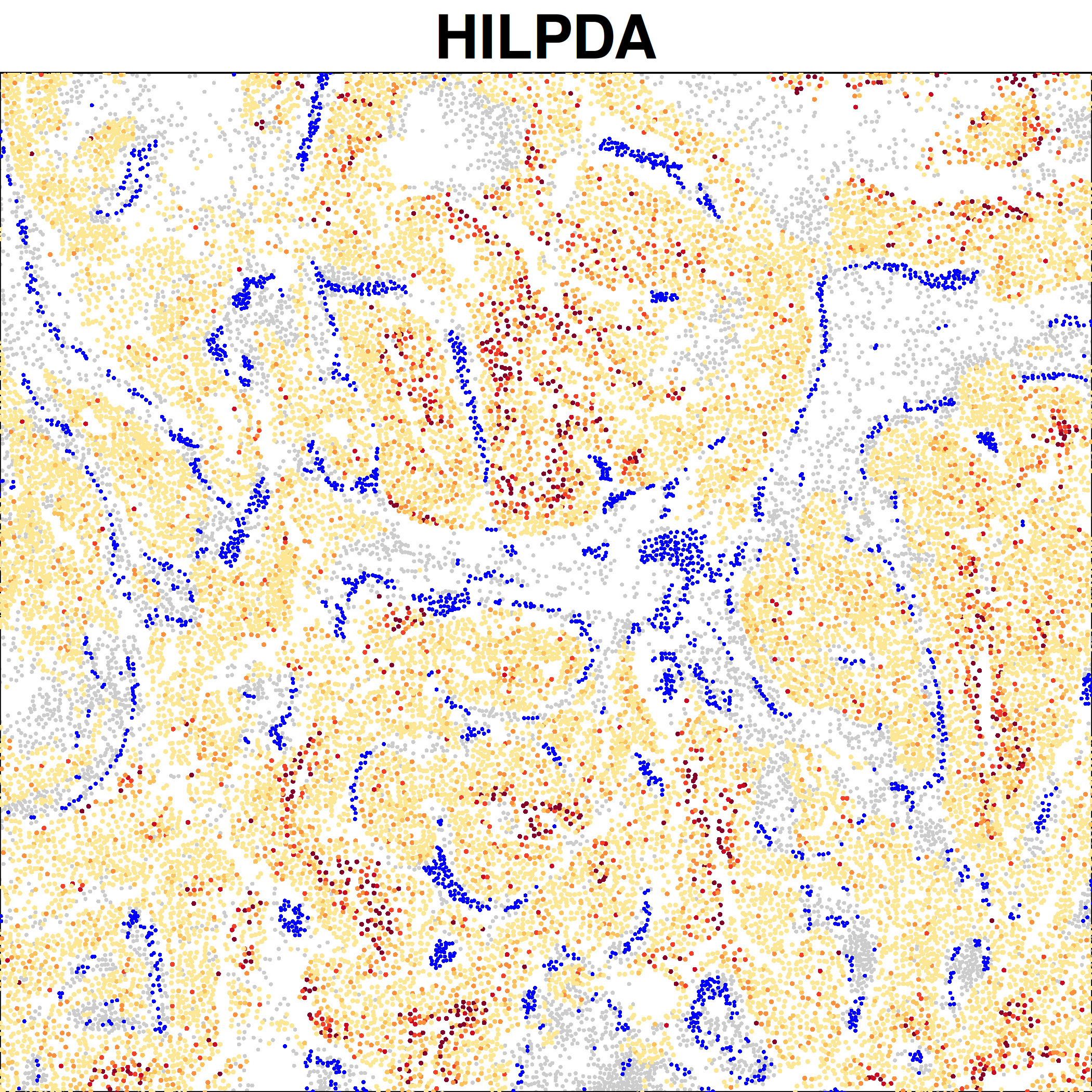
We choose a handful of genes of interest and show how they change over distance, as well as making spatial plots to show their expression.
Show the code
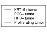
#### mean selected gene expression over distance:# get matrix of mean expression per bin:mat <-readRDS(paste0(vessel_dir, "/Data/top1000_tumorExp_byVesselDist_expr_wide_matrix.rds"))# remove LUM+, also known as IGTB6+:mat <- mat[, !grepl("LUM", colnames(mat))]matbin <-as.numeric(substr(colnames(mat), unlist(gregexpr("_", colnames(mat))) +1, nchar(colnames(mat))))# set up plots:subtypenames <-paste0(c("KRT16+", "PGC+", "HPD+", "Proliferating"), " tumor")clustcols <-c("blueviolet", "brown1", "grey20", "steelblue3")names(clustcols) <- subtypenamesfor (gene inc("AZGP1", "HILPDA", "PLA2G2A", "ELF3", "VEGFA")) {svg(paste0(vessel_dir, "/Plots/trend - ", gene, ".svg"), width =3, height =3)par(mar =c(4,4,0,0))plot(0,0,col=0,xlim =range(matbin), ylim =range(mat[gene, ]),xlab ="mm to vessel", ylab = gene)for (cell in subtypenames) { cellinds <-grepl(make.names(cell), make.names(colnames(mat)))lines(matbin[cellinds], mat[gene, cellinds], col = clustcols[cell]) }dev.off()}svg(paste0(vessel_dir, "/Plots/trend - legend.svg"), width =2.2, height =1.5)par(mar =c(0,0,0,0))frame()legend("center", lty =1, col = clustcols, legend =names(clustcols))dev.off()
Line plots showing expression over vessel distance: