8  Low-proliferation zones

Here we characterize regions of low cancer cell profliferation.

8.1 Assign proliferation scores

We start by assigning proliferation scores to each cell, using Seurat’s cell cycle scoring method.

Next, we load in basic data.

library(data.table) 
library(InSituCor)
library(scales)
library(pheatmap)
library(RColorBrewer)
library(smiDE)
library(fgsea)  
library(dplyr)
library(alphahull)
library(Seurat)
library(SeuratObject)

source("patchDE utils.R")

#### load data ------------------------------

raw <- Matrix::t(readRDS(paste0(analysis_dir, "/Robjects/raw_exp_mat.rds")))
xy <- readRDS(paste0(analysis_dir, "/Robjects/xy.rds"))
clustdf <- readRDS(paste0(analysis_dir, "/Robjects/cell_types.rds"))
clust <- clustdf$major_cell_type
iscancer <- clust == "Tumor"
cellcycle <- readRDS(paste0(prolif_dir, "/Data/cell_cycle_predictions.rds"))
cellcyclecanceronly <- replace(cellcycle, !iscancer, "notcancer")
niches <- readRDS(paste0(analysis_dir, "/niches/Data/novae_domains_9_assignments.rds"))
seu <- readRDS(paste0(analysis_dir, "/Robjects/seurat_object_postCellTyping.rds"))
annot <- seu@meta.data
stopifnot(identical(annot$cell_ID, rownames(raw)))
rm(seu)
annot$celltype <- clust

# rotated xy:
xy21 <- xy[, 2:1]
xy21[, 2] <- mean(xy21[, 2]) - xy21[, 2]

Now we’ll partition the tissue into regions of high/low tumor proliferation:

# there are islands of G1 phase, otherwise cancer cells are mostly G2/M/S... what explains the islands where it's failing to proliferate?
if (!file.exists(paste0(prolif_dir, "/Data/neighbors100.RDS"))) {
  neighbors100 <- InSituCor:::nearestNeighborGraph(x = xy[, 1], y = xy[, 2], N = 100)
  saveRDS(neighbors100, file = paste0(prolif_dir, "/Data/neighbors100.RDS"))
} else {
  neighbors100 <- readRDS(paste0(prolif_dir, "/Data/neighbors100.RDS"))
}

if (!file.exists(paste0(prolif_dir, "/Data/neighborhoodcelltypes.RDS"))) {
  # neighbor counts of tumor cells in each cell cycle phase
  nphase <- InSituCor:::neighbor_tabulate(cellcyclecanceronly, neighbors100) 
  # neighbor counts of cell types:
  neighborhoodcelltypes <- InSituCor:::neighbor_tabulate(clust, neighbors100) 
  saveRDS(nphase, file = paste0(prolif_dir, "/Data/nphase.RDS"))
  saveRDS(neighborhoodcelltypes, file = paste0(prolif_dir, "/Data/neighborhoodcelltypes.RDS"))
} else {
  nphase <- readRDS(paste0(prolif_dir, "/Data/nphase.RDS"))
  neighborhoodcelltypes <- readRDS(paste0(prolif_dir, "/Data/neighborhoodcelltypes.RDS"))
}
rm(neighbors100)

# rate of proliferating cancer cells in neighborhood:
prop_g2ms <- rowSums(nphase[, c("G2M", "S")]) / rowSums(nphase[, c("G1", "G2M", "S")])
prop_g2ms[is.na(prop_g2ms)] <- 0
# number of cancer cells in neighborhood:
ncancer_all <- rowSums(nphase[, c("G1", "G2M", "S")])
ncancer_cycling <- rowSums(nphase[, c("G2M", "S")])
ncancer_resting <- nphase[, "G1"]


#### What characterizes cancer cells in highly proliferative regions? -------------

# classify cancer cells as occupying proliferative/quiescent regions:
use <- (clust == "Tumor") & (ncancer_all >= 20) 
hist(prop_g2ms[use], breaks = 25)
abline(v = 0.5, col = 2)
prolifcat <- c("quiescent", "proliferative")[1 + (prop_g2ms > 0.5)]

## summarize tumor proliferation context:
table(prolifcat[iscancer]) / sum(table(prolifcat[iscancer]))

# polygons around quiescent areas:
dbuse <- (prolifcat == "quiescent") & (iscancer)
db <- dbscan::dbscan(xy[dbuse, ], eps = 0.05, minPts = 20)
if (!file.exists(paste0(prolif_dir, "/Data/qpolys.RDS"))) {
  qpolys <- list()
  for (i in setdiff(unique(db$cluster), 0)) {
    if (i %% 10 == 0){print(i)}
    inds <- which(dbuse)[db$cluster == i]
    qpolys[[as.character(i)]] <- alphahull::ahull(xy21[inds, ], alpha = 0.04)

    arcs <- qpolys[[as.character(i)]]$arcs
    arcs_clean <- arcs[(arcs[, "r"] > 0) & (arcs[, "end1"] != arcs[, "end2"]), ]
    qpolys[[as.character(i)]]$arcs <- arcs_clean
  }
  saveRDS(qpolys, file = paste0(prolif_dir, "/Data/qpolys.RDS"))
} else {
  qpolys <- readRDS(paste0(prolif_dir, "/Data/qpolys.RDS"))
}

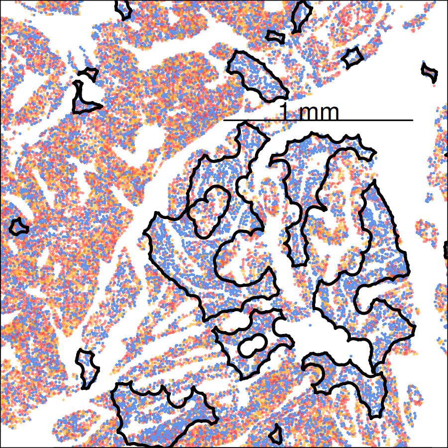
# show the cell type results and the classification:
inds <- clust == "Tumor"
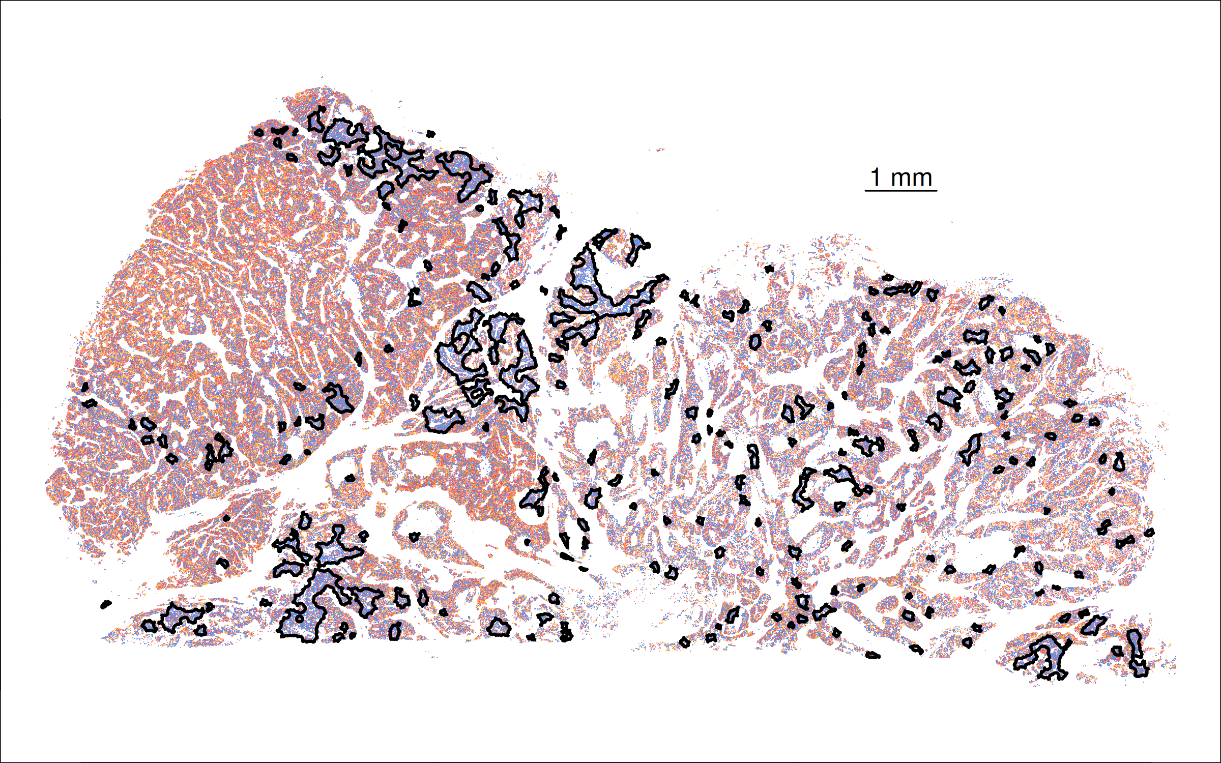
cccols <- c("G1" = "cornflowerblue", "G2M" = scales::alpha("orange", 0.5), "S" = scales::alpha("firebrick1", 0.5))
png(paste0(prolif_dir, "/Plots/cellcycle - whole tissue.png"), width =8, height = 5, units = "in", res = 300)
par(mar = c(0,0,0,0))
plot(xy21[inds, ], pch = 16, cex = 0.1, asp = 1, col = cccols[cellcycle[inds]])
lines(c(11,12), c(3,3))
text(11.5, 3.2, "1 mm")
for (i in 1:length(qpolys)) {
  plot(qpolys[[i]], add = TRUE, wpoints = F, col = "black")
}
dev.off()
svg(paste0(prolif_dir, "/Plots/cellcycle color legend.svg"), width = .7, height = .8)
par(mar = c(0,0,0,0))
frame()
legend("center", pch = 16, col = cccols, legend = names(cccols))
dev.off()

png(paste0(prolif_dir, "/Plots/cellcycle - zoomed.png"), width = 3, height = 3, units = "in", res = 300)
par(mar = c(0,0,0,0))
plot(xy21[inds, ], pch = 16, cex = 0.25, asp = 1, col = cccols[cellcycle[inds]],
     xlim = c(4.3,6.5), ylim = c(-0.2, 1.8))
lines(c(5.4,6.4), c(1.35,1.35))
text(5.85, 1.4, "1 mm")
for (i in 1:length(qpolys)) {
  plot(qpolys[[i]], add = TRUE, wpoints = F, col = "black")
}
dev.off()

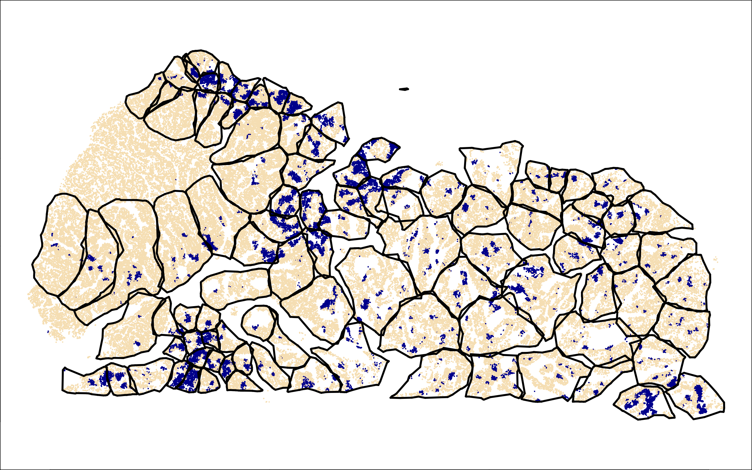
Now we run the PatchDE algorithm to partition the tissue into patches to be analyzed separately:

use <- ((clust == "Tumor") & (ncancer_all >= 20)) & (cellcycle == "G1")
Xall <- model.matrix(lm(rnorm(length(prolifcat)) ~ prolifcat))

# run it:
if (!file.exists(paste0(prolif_dir, "/Data/patchDE.RDS"))) {
  set.seed(0)
  res <- getPatches(xy = xy[use, 2:1], 
                    X = Xall[use, 2], 
                    npatches = 100,
                    bitesize = 0.1,
                    maxradius = 5,
                    roundness = 0.25,
                    initwithhotspots = TRUE,
                    n_iters = 10,
                    alpha = 0.5,
                    effectivezerodist = 0.025,
                    plotprogress = TRUE) 
    
  saveRDS(res, file = paste0(prolif_dir, "/Data/patchDE.RDS"))
} else {
  res <- readRDS(paste0(prolif_dir, "/Data/patchDE.RDS"))
}

barplot(table(prolifcat[use], res[use])[2:1, ], ylim = c(0,100))

polys <- getPatchHulls(xy21[use, ], patch = res, alpha = 0.3) 

png(paste0(prolif_dir, "/Plots/patchDE bins2.png"), width =8, height = 5, units = "in", res = 300)
par(mar = c(0,0,0,0))
plot(xy21[use, ], pch = 16, cex = 0.2, asp = 1,
     col = c("wheat", "darkblue")[as.numeric(as.factor(prolifcat[use]))])
for (i in 1:length(polys)) {
  if (!is.null(polys[[i]])) {
    plot(polys[[i]], add = TRUE, wpoints = F)#, col = "black")  
  }
}
dev.off()

Now we lay the groundwork for DE:

if (!file.exists(paste0(prolif_dir, "/Data/overlap_metrics.rds"))) {
  overlap_metrics <-
    smiDE::contamination_ratio_metric(assay_matrix = Matrix::t(raw),
                                      metadata = annot,
                                      cluster_col = "celltype",
                                      radius = 0.05,
                                      sdimx_col = "x_slide_mm",
                                      sdimy_col = "y_slide_mm"
    )
  # Save overlap metrics
  saveRDS(overlap_metrics, file = paste0(prolif_dir, "/Data/overlap_metrics.rds"))
} else {
  overlap_metrics <- readRDS(paste0(prolif_dir, "/Data/overlap_metrics.rds"))
}

## set up DE:
scaling_factors <- Matrix::rowSums(raw)
norm <- Matrix::Diagonal(x = scaling_factors^-1) %*% raw * mean(scaling_factors)

# which genes to keep: low overlap, not low mean
analysis_genes <- overlap_metrics[celltype == "Tumor" & (ratio <= 1)]$target
length(analysis_genes)
norm <- norm[, analysis_genes]

# scale norm:
genefactors <- pmax(Matrix::colMeans(norm), 0.1)
genefactors <- genefactors / mean(genefactors)
norm.s <- norm %*% Matrix::Diagonal(x = 1 / genefactors)
colnames(norm.s) <- colnames(norm)

Now we run DE over each patch:

if (!file.exists(paste0(prolif_dir, "/Data/patchDEresults.RDS"))) {
  deres <- patchDE(y = norm.s[use, ], df = data.frame(prolifcat = prolifcat[use]), patch = res)
  saveRDS(deres, file = paste0(prolif_dir, "/Data/patchDEresults.RDS"))
} else {
  deres <- readRDS(paste0(prolif_dir, "/Data/patchDEresults.RDS"))
}


# replace NA results - arising from all-0 expression - with 0s:
ps <- replace(deres$prolifcatquiescent$pvals, is.na(deres$prolifcatquiescent$pvals), 1)
ests <- replace(deres$prolifcatquiescent$ests, is.na(deres$prolifcatquiescent$pvals), 0)
ses <- replace(deres$prolifcatquiescent$ses, is.na(deres$prolifcatquiescent$pvals), 1e6)

# write supplementary table of DE results:
out <- data.table(gene = rep(rownames(ps), ncol(ps)),
                  patch = rep(colnames(ps), each = nrow(ps)),
                  estimate = as.vector(ests),
                  pvalue = as.vector(ps),
                  se = as.vector(ses))
write.csv(out, file = paste0(prolif_dir, "/Data/Supplementary table - patchDE results.csv"))

# ID noteworthy genes:
eps <- 0.5
crit <- (abs(ests) > eps) & (ps < 0.01)
critdir <- 1*((ests > eps) & (ps < 0.01)) - 1*((ests < -eps) & (ps < 0.01))
list1 <- names(which(rowSums(crit) >= 3))

Now let’s explore our results:

# how widespread were the hits?
sum(rowSums(ps[list1, ] < 0.01) < 0.5*ncol(ps))
sum(rowSums(ps[list1, ] < 0.01) < 0.1*ncol(ps))
hist(rowMeans(ps[list1, ] < 0.01))


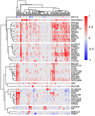
# cluster the genes:
cormat <- cor(t(ests[list1, ]))

p1 <- pheatmap::pheatmap((ests * (ps < 0.05))[list1, ], 
               breaks = seq(-1,1,length.out=101),
               fontsize_row = 8, show_colnames = F,
               cutree_rows = 10,
               clustering_distance_rows = "correlation",
               border_color = NA,
               color = colorRampPalette(c("blue", "grey90", "red"))(100))

cuts <- cutree(p1$tree_row, k = 10)

svg(paste0(prolif_dir, "/Plots/patchDE heatmap by tiny bin.svg"), height = 5.5, width = 4.5)
print(p1)
dev.off()
#png("results/patchDE heatmap by tiny bin - tall.svg", height = 8, width = 3.5, units = "in", res = 400)\
svg(paste0(prolif_dir, "/Plots/patchDE heatmap by tiny bin - tall.svg"), height = 10, width = 3.5)
print(p1)
dev.off()

# make metagenes:
unique_cuts <- unique(cuts)
result_list <- vector("list", length(unique_cuts))
names(result_list) <- unique_cuts
for (i in seq_along(unique_cuts)) {
  cutnum <- unique_cuts[i]
  tempgenes <- names(cuts)[cuts == cutnum]
  result_list[[i]] <- Matrix::rowMeans(norm.s[, tempgenes, drop = FALSE])
}

mscores <- do.call(cbind, result_list)
colnames(mscores) <- unique_cuts
for (i in 1:ncol(mscores)) {
  colnames(mscores)[i] <- substr(paste0(names(cuts[cuts == i]), collapse = "_"), 1, 20)
}

# how often is the major metagene significant?
genes <- names(cuts)[cuts == 2]
rowMeans(ps[genes, ] < 1e-2)

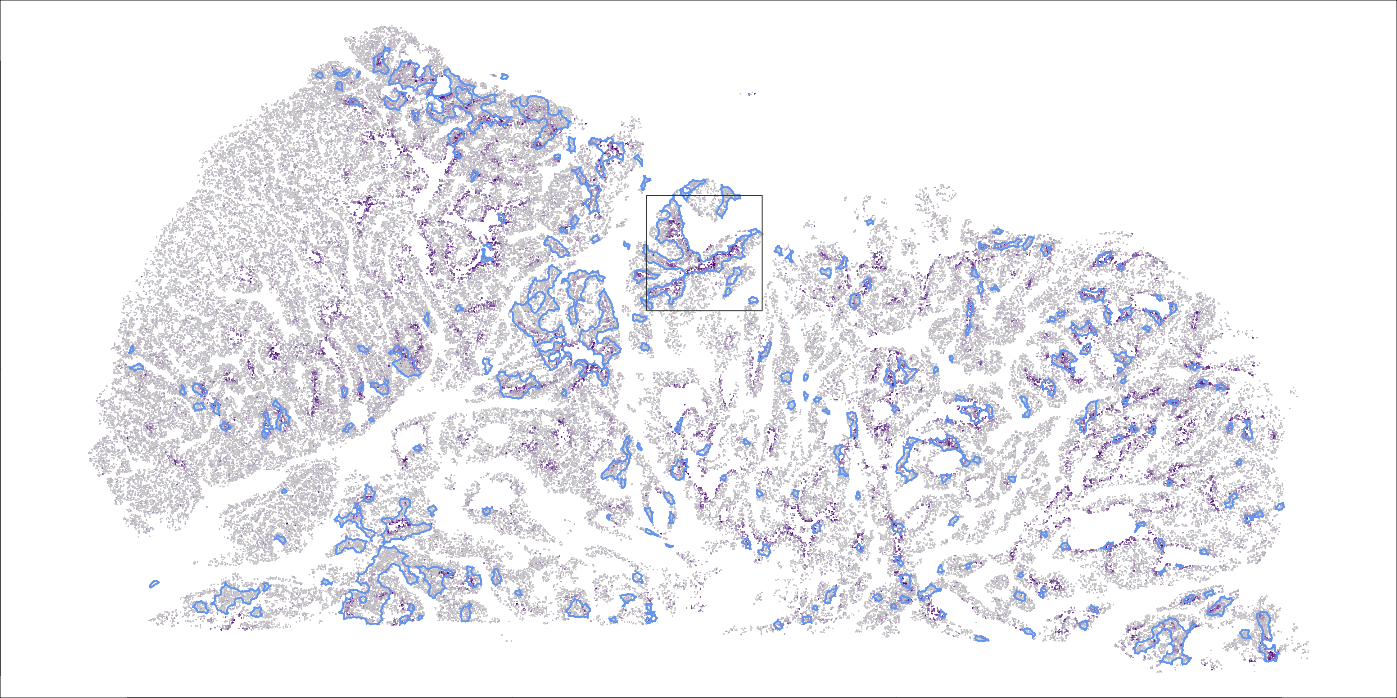
## customized plots for 2 selected metagenes:
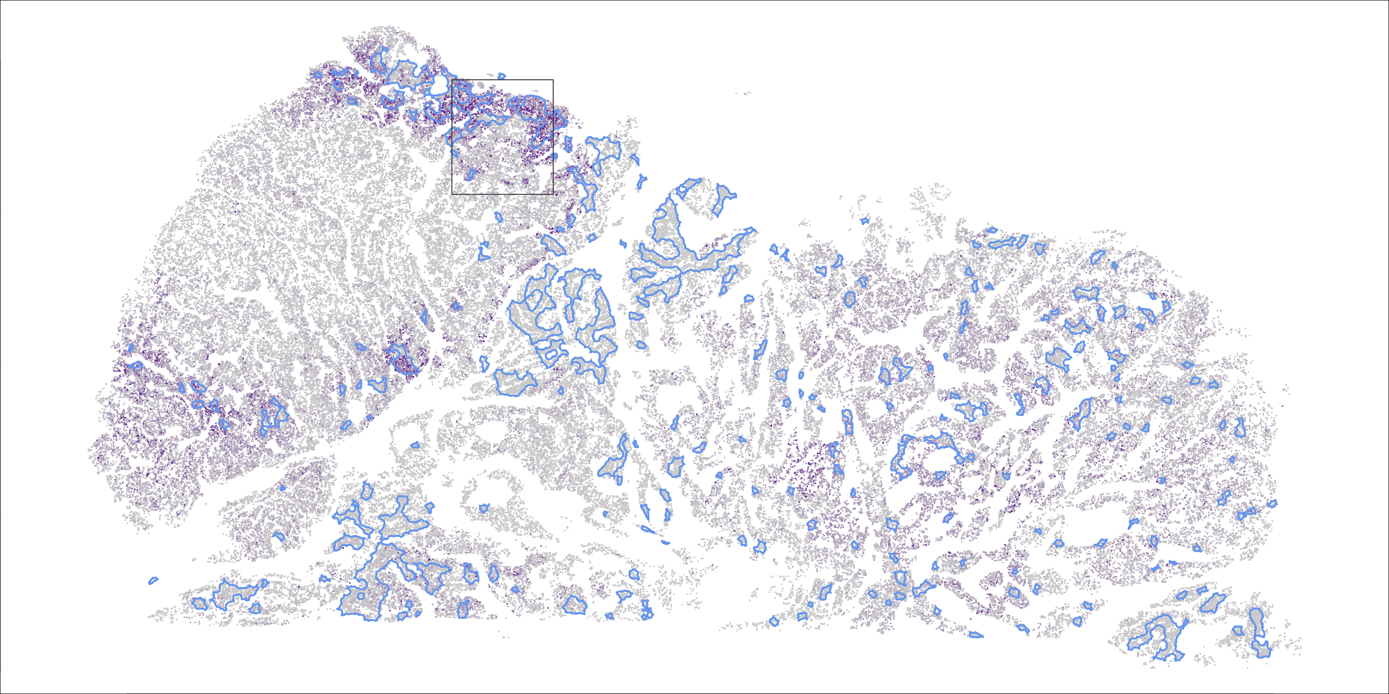
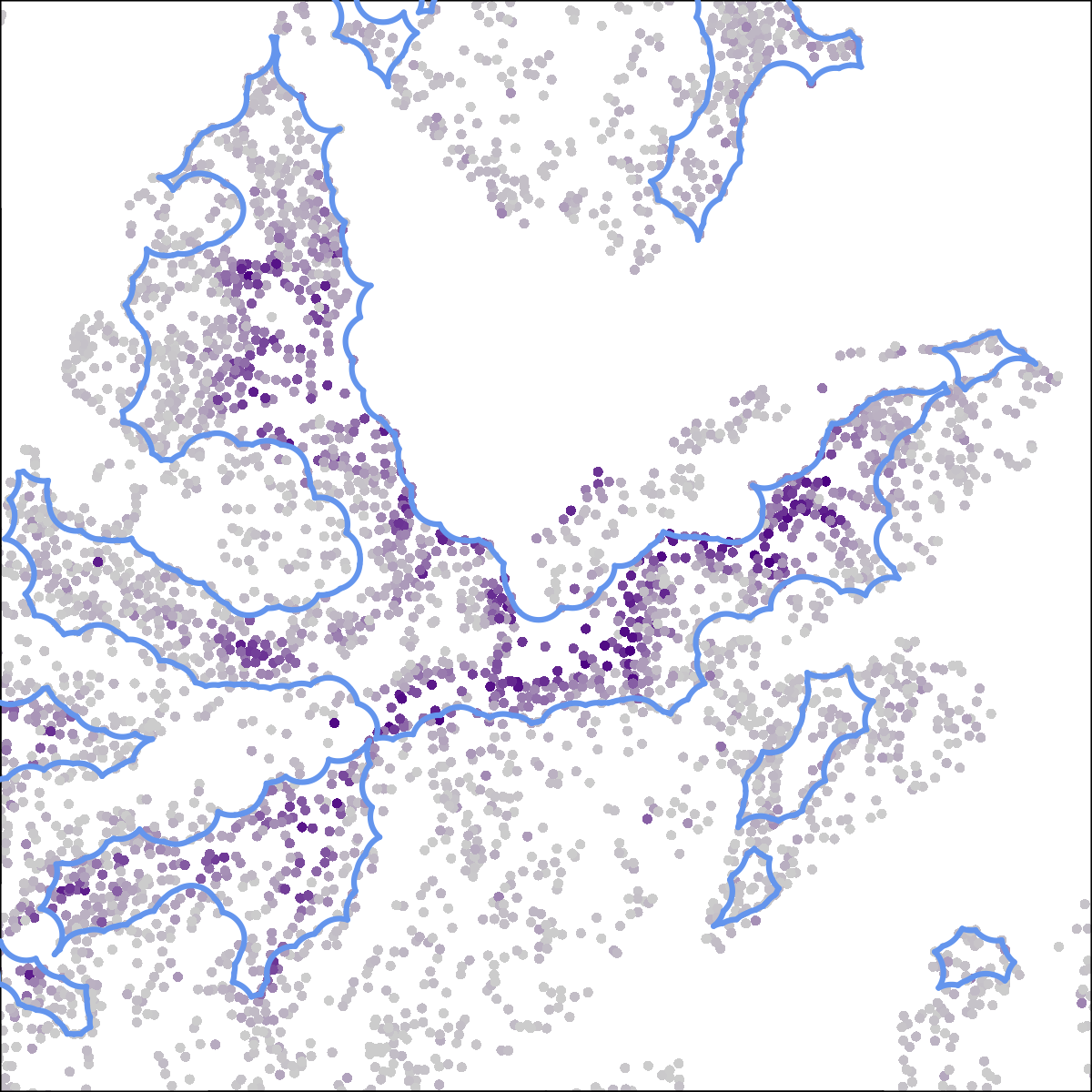
name = "ADM_ANGPTL4_BNIP3_EG"
xlim = c(6.75,8.25); ylim = c(0.75,2.25)
png(paste0(prolif_dir, "/Plots/patchDE metagene ", name,".png"), 
    res = 300, units = "in", width = 15, height = 7.5)
par(mar = c(0,0,0,0))
plot(xy21[use, ], pch = 16, cex = 0.25, asp = 1,
     col = colorRampPalette(c("grey80", "#4B0082"))(100)[
       round(1 + 100 * pmin(mscores[, name][use] / quantile(mscores[, name][use], 0.995), 1))
     ])
for (i in 1:length(qpolys)) {
  plot(qpolys[[i]], add = TRUE, wpoints = F, 
       col = "cornflowerblue")
}
rect(xlim[1], ylim[1], xlim[2], ylim[2], border = "grey20")
dev.off()

png(paste0(prolif_dir, "/Plots/patchDE zoomed metagene ", name,".png"), 
    res = 300, units = "in", width = 4, height = 4)
par(mar = c(0,0,0,0))
plot(xy21[use, ], pch = 16, cex = 0.5, asp = 1,
     col = colorRampPalette(c("grey80", "#4B0082"))(100)[
       round(1 + 100 * pmin(mscores[, name][use] / quantile(mscores[, name][use], 0.995), 1))
     ],
     xlim = xlim, ylim = ylim)
for (i in 1:length(qpolys)) {
  plot(qpolys[[i]], add = TRUE, wpoints = F, 
       col = "cornflowerblue")
}
dev.off()


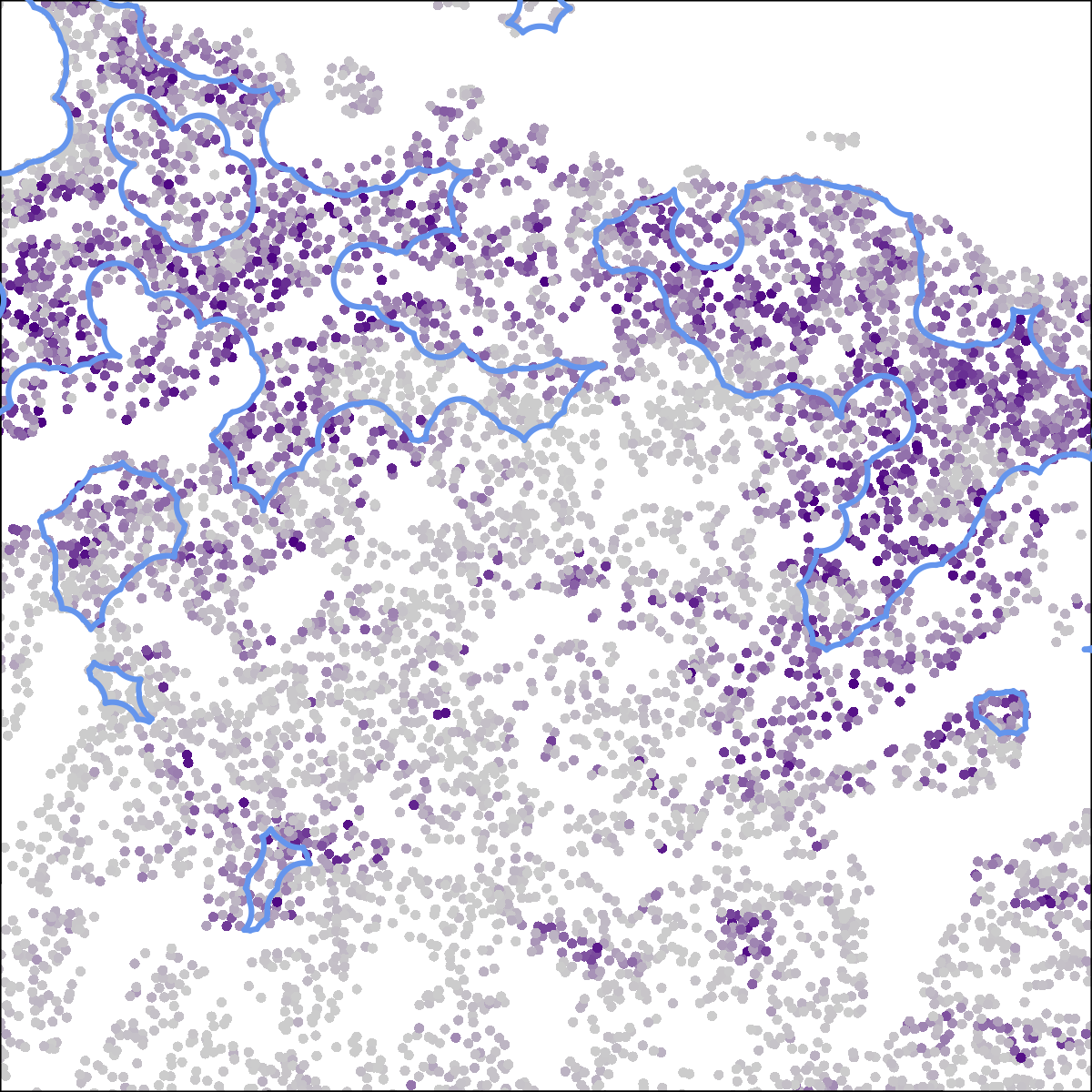
name = "CYP4F8_PIP"
xlim = c(4.25, 5.575); ylim = c(2.25,3.75)
png(paste0(prolif_dir, "/Plots/patchDE metagene ", name,".png"), 
    res = 300, units = "in", width = 15, height = 7.5)
par(mar = c(0,0,0,0))
plot(xy21[use, ], pch = 16, cex = 0.25, asp = 1,
     col = colorRampPalette(c("grey80", "#4B0082"))(100)[
       round(1 + 100 * pmin(mscores[, name][use] / quantile(mscores[, name][use], 0.995), 1))
     ])
for (i in 1:length(qpolys)) {
  plot(qpolys[[i]], add = TRUE, wpoints = F, 
       col = "cornflowerblue")
}
rect(xlim[1], ylim[1], xlim[2], ylim[2], border = "grey20")
dev.off()
png(paste0(prolif_dir, "/Plots/patchDE zoomed metagene ", name,".png"), 
    res = 300, units = "in", width = 4, height = 4)
par(mar = c(0,0,0,0))
plot(xy21[use, ], pch = 16, cex = 0.5, asp = 1,
     col = colorRampPalette(c("grey80", "#4B0082"))(100)[
       round(1 + 100 * pmin(mscores[, name][use] / quantile(mscores[, name][use], 0.995), 1))
     ],
     xlim = xlim, ylim = ylim)
for (i in 1:length(qpolys)) {
  plot(qpolys[[i]], add = TRUE, wpoints = F, 
       col = "cornflowerblue")
}
dev.off()