8 Differential Expression

source("./preamble.R")
library(ggplot2)
library(stringr)
reticulate::source_python("./preamble.py")
analysis_dir <- file.path(getwd(), "analysis_results")
input_dir <- file.path(analysis_dir, "input_files")
output_dir <- file.path(analysis_dir, "output_files")
analysis_asset_dir <- "./assets/analysis_results"
ct_dir <- file.path(output_dir, "ct")
de_dir <- file.path(output_dir, "de")
if(!dir.exists(de_dir)){
  dir.create(de_dir, recursive = TRUE)
}
results_list_file = file.path(analysis_dir, "results_list.rds")
if(!file.exists(results_list_file)){
  results_list <- list()
  saveRDS(results_list, results_list_file)
} else {
  results_list <- readRDS(results_list_file)  
}

library(smiDE)

8.1 Introduction

There are several points during exploratory data analysis were observations turn into biologicaly hypotheses. Often times we want to convert a given biological hypothesis into a statistical one to formally test for differences between two or more groups. Differential Expression (DE) analysis is one such tool that allows us to test these hypotheses. In this chapter we’ll run differential expression analysis using the smiDE R package that was specifically designed to account for the spatial relationship found in CosMx SMI data. We’ll continue to work with the colon cancer dataset where we previously identified two tumor-rich spatial domains – the Tumor Core and the Desmoplastic Stroma – with varying levels of PROGENy pathway enrichment scores.

There are many ways one could go about using smiDE and enumerating all the ways is beyond the scope of this chapter. Let’s consider two motivating questions centered around the tumor cells themselves:

1. Location based: How are tumor cells’ expression influenced by the domain in which they reside? Here the grouping variable will be the annotated domain a tumor cell belongs to.
2. “Immune Pressure” based: How are tumor cells’ expression influenced by the number of spatially adjacent immune cells? In this case, the grouping variable will be a numeric value (e.g., a given tumor cell might have 10 immune cells within a given spatial radius while another tumor cell might have zero immune cells nearby).

Most of this chapter will be based in R and so we’ll first convert our annData object before we tackle these questions. For each DE question there will be a lot of results to look at and the smiDE package has ways to evaluate and explore these results. Instead of enumerating all the volcano plots and other results here, I will show how I loaded them into the Differential Expression Explorer Browser Byte Dashboard.

8.2 Converting Data

Read the annData object.

if 'adata' not in dir():
  filename = os.path.join(r.analysis_dir, "anndata-7-domain_annotations.h5ad")
  adata = ad.read_h5ad(filename)

counts = adata.layers['counts'].astype('int64')
norm = adata.layers['TC']

Before we switch over to R for DE, let’s calculate the number of immune cells within 80 microns of a tumor cell. We’ll use this information for the second DE question. We’ll create a KDtree of the immune cells and then query all of the cells in the annData object to tally the number of adjacent immune cells within 80 microns.

from sklearn.neighbors import KDTree
import numpy as np
import pandas as pd

radius_mm = 0.080
cell_type_column = "celltype_broad"
immune_cell_types = [
    "bcell", "dendritic", "macrophage", "mast", 
                  "mix_NK_Lymphoid", "monocyte", "neutrophil", "nk", "plasma", "tcell"
]

coords = adata.obsm['spatial']
is_immune = adata.obs[cell_type_column].isin(immune_cell_types).values
immune_coords = coords[is_immune]
tree = KDTree(immune_coords)
# Query all cells
tally = tree.query_radius(coords, r=radius_mm, count_only=True)
# If the focal cell itself is immune, subtract 1 from the total
final_tally = tally - is_immune.astype(int)
adata.obs['n_ct_immune_neighbors'] = final_tally

Now switch to R and load and “munge” the data.

counts_mat <- Matrix::t(py$counts)
colnames(counts_mat) <- py$adata$obs_names$to_list()
rownames(counts_mat) <- py$adata$var_names$to_list()

norm_mat <- Matrix::t(py$norm)
colnames(norm_mat) <- py$adata$obs_names$to_list()
rownames(norm_mat) <- py$adata$var_names$to_list()

meta_df <- py$adata$obs
rownames(meta_df) <- meta_df$cell_id_numeric <- colnames(counts_mat)

totalcount_scalefactors <- mean(meta_df[["nCount_RNA"]]) / meta_df[["nCount_RNA"]]
names(totalcount_scalefactors) <- rownames(meta_df)

xy <- py$adata$obsm['spatial']
colnames(xy) <- c("sdimx", "sdimy")
meta_df <- cbind(meta_df, xy)

8.3 Setup

There are a few cells that do not have a spatial domain assignment. These are labeled as missing values which isn’t allowed for smiDE. Therefore, subset the expression matrices and metadata to include only cells with spatial domains.

cells_use <- !is.na(meta_df$annotated_domain)
meta_use <- meta_df[cells_use,]
counts_mat_use <- counts_mat[,cells_use]
norm_mat_use <- norm_mat[,cells_use]

8.3.1 Overlap Ratio Metric

We want to exclude any gene targets that might be from abutting cells that are not tumor cells. For example, JCHAIN is often highly expressed in plasma cells, so we might see JCHAIN spuriously show up as higher in tumor cells in a domain with a high abundance of plasma cells. The function below mitigates that effect by considering the gene expression of a focal cell relative to close neighbors who are not of the same cell type. See the documentation here and the Choosing an overlap ratio deep-dive box below for more details. We’ll select genes that have a ratio of less than 1.

overlap_metrics <- smiDE::overlap_ratio_metric(assay_matrix = norm_mat_use,
                                  metadata = meta_use,
                                  cellid_col = "cell_id_numeric",
                                  cluster_col = "celltype_broad",
                                  sdimx_col = "sdimx",
                                  sdimy_col = "sdimy",
                                  radius = 0.05
                                  )

genes_to_analyze <- overlap_metrics[celltype_broad=="tumor"][ratio < 1][["target"]]
saveRDS(genes_to_analyze, file=file.path(de_dir, "genes_to_analyze.rds"))

Choosing an overlap ratio

We can define the intrinsic expression of a cell type as the collection of gene targets demonstrating consistently higher expression within that focal cell type compared to its immediate spatial neighbors. Because pervasive, uniform gene translation across all cells is biologically improbable, spatial differential expression (DE) models can account for this localized specificity.

To quantify this localized specificity, we establish an empirical overlap ratio for each target-by-cell-type combination (e.g., Gene A in Cell Type B). For a given gene, this statistic is calculated by taking its average expression in non-focal cells and dividing it by its average expression in the focal cell type.

Leveraging these local spatial patterns prior to DE analysis provides a systematic way to:

• Filter spurious signals: Identify genes whose expression is primarily bleeding over from adjacent cells.
• Reduce the multiple testing burden: Limit the number of hypotheses (targets) we test to those with true biological relevance in the cells of interest.

Specifically, targets driven heavily by neighboring non-focal cells (such as fibroblasts or NK cells) will yield a ratio > 1. For analytical clarity, this overlap is typically evaluated in log space, where expression predominantly originating from the non-focal neighborhood corresponds to a log2(ratio) > 0.

overlap_metrics$log2ratio <- log2(overlap_metrics$ratio)

Let’s explore how this transformed ratio behaves. We’ll compute the empirical cummulative distribution function (eCDF) for each focal cell type that is in the overlap_metrics R object. We do this simply by grouping by cell type, sorting the results, and then returning the proportion of targets that have a smaller ratio.

ecdf <- do.call(rbind, lapply(unique(overlap_metrics[['celltype_broad']]), function(fct){
              x <- overlap_metrics[overlap_metrics[['celltype_broad']]==fct,]
              x <- x[order(x[['log2ratio']]),]
              return(
                data.frame(focal_cell_type = x[['celltype_broad']],
                           target=x[['target']], log2ratio = x[['log2ratio']],
                           prop = (1:nrow(x)) / nrow(x))
              )
            }))
saveRDS(ecdf, file=file.path(de_dir, "ecdf.rds"))

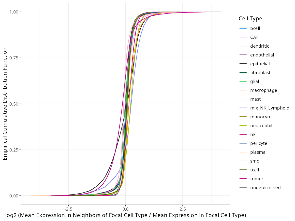
And here is what those eCDFs look like.

celltype_broad_colors <- results_list[['celltype_broad_colors']]
names(celltype_broad_colors) <- results_list[['celltype_broad_names']]

p <- ggplot() +
              geom_line(data=ecdf,
                        aes(x=log2ratio, y=prop, colour=focal_cell_type, group=focal_cell_type)) +
              theme_bw() +
      scale_color_manual(values=celltype_broad_colors) + 
              xlab("log2 (Mean Expression in Neighbors of Focal Cell Type / Mean Expression in Focal Cell Type)") +
              ylab("Empirical Cumulative Distribution Function") +
              guides(colour=guide_legend(title="Cell Type"))

ggsave(p, filename=file.path(de_dir, "ecdfs.png"),
       width=8, height=6, dpi=150, type="cairo")

Figure 8.1: Empirical cummulative distribution for each cell type. Y proportion of gene targets have a log2 ratio less than X.

You can see from Figure 8.1 that the proportion of targets that are more abundant in a given cell type relative to other cell types depends on the cell type. If we look only at X = 0, we see the proportion of targets that have higher intrinsic expression for each cell type. Those values are shown in table Table 8.1.

ecdf_at_zero <- ecdf %>%
  group_by(focal_cell_type) %>%
  summarize(
    prop_at_zero = approx(x = log2ratio, y = prop, xout = 0)$y
  ) %>% arrange(prop_at_zero)

ecdf_at_zero$targets_below_zero <- round(ecdf_at_zero$prop_at_zero * length(unique(ecdf$target)))

saveRDS(ecdf_at_zero, file=file.path(de_dir, "ecdf_at_zero.rds"))

Table 8.1: Approximate number of targets that have focal cell type expression that is greater than neighboring non-focal cell type expression.

Cell Type	Prop. Targets below log2(ratio) = 0	Total Targets below log2(ratio) = 0
neutrophil	0.1940	3,674
plasma	0.2348	4,445
monocyte	0.2475	4,686
mix_NK_Lymphoid	0.2529	4,789
nk	0.2549	4,827
macrophage	0.2993	5,667
mast	0.3367	6,376
tcell	0.3367	6,376
dendritic	0.3568	6,755
fibroblast	0.3740	7,082
CAF	0.3833	7,257
pericyte	0.3837	7,266
bcell	0.4128	7,817
glial	0.4452	8,430
epithelial	0.4620	8,749
endothelial	0.4757	9,007
undetermined	0.5345	10,120
tumor	0.6497	12,303
smc	0.6900	13,065

For our cell type of interest, tumor, we see that the number of intrinsic expression is 12,303 targets. And what about our intuition about JCHAIN in tumor? The log2 ratio of JCHAIN in tumor is 2.02 (ratio = 4.07) and that is more extreme than 99% of targets. In plasma cells, on the other hand, the log2 ratio of JCHAIN is -2.80 (ratio = 0.14) which happens to be the lowest ratio for plasma cells which makes biological sense.

ecdf <- readRDS(file.path(de_dir, "ecdf.rds"))
filter(ecdf, focal_cell_type %in% c("tumor", "plasma"), target=="JCHAIN")

  focal_cell_type target log2ratio         prop
1          plasma JCHAIN -2.800541 5.281225e-05
2           tumor JCHAIN  2.026144 9.941907e-01

In this chapter we chose a log2 ratio of < 0 (ratio < 1). In practice that threshold is a good “rule of thumb” but the choice is entirely up to the user. Here’s an eCDF plot that focuses on tumor only. The rug above the x-axis shows the relative density of targets. Hover over the plot to more detail.

ecdf_file <- "./assets/interactives/ecdf.parquet"
nanoparquet::write_parquet(ecdf %>% filter(focal_cell_type == "tumor") %>% select(-focal_cell_type), ecdf_file)

db = DuckDBClient.of({
  ecdf_data: FileAttachment("assets/interactives/ecdf.parquet")
})

// Query data from DuckDB
raw_data = db.sql`SELECT * FROM ecdf_data ORDER BY log2ratio ASC`

// Format data for Plot
plotData = raw_data.map((d, i) => ({
  ...d,
  // Force numeric types to prevent "scale incompatible" errors
  log2ratio: Number(d.log2ratio),
  prop: Number(d.prop),
  count_less: i 
}))

// Render the eCDF Chart
chart = Plot.plot({
  width: 800,
  height: 500,
  x: { 
    label: "Log2 Ratio", 
    type: "linear" 
  },
  y: { 
    label: "Proportion", 
    type: "linear" 
  }, 
  marks: [
    // 1. The Binned Rug Plot (Optimized for 20k rows)
    Plot.ruleX(plotData, Plot.binX(
      { strokeOpacity: "count" }, 
      {
        x: "log2ratio",
        y1: 0,             // Start at X-axis
        y2: 0.03,          // 3% tick height
        strokeWidth: 3,
        thresholds: 200   
      }
    )),

    // 2. The main eCDF line
    Plot.line(plotData, {
      x: "log2ratio", 
      y: "prop", 
      stroke: "#C11A7A",
      strokeWidth: 2.5
    }),
    
    // 3. The constrained vertical drop-line on hover
    Plot.ruleX(plotData, Plot.pointerX({
      x: "log2ratio",
      y1: 0,         
      y2: "prop",    
      stroke: "gray",
      strokeDasharray: "4,4",
      strokeWidth: 1.5
    })),
    
    // 4. The Hover Tooltip (with rounded formatting)
    Plot.tip(plotData, Plot.pointerX({
      x: "log2ratio", 
      y: "prop", 
      // Using .toFixed() and .toPrecision() to format the long decimals
      title: d => `Target: ${d.target}\nTargets < Y: ${d.count_less}\nLog2 Ratio: ${d.log2ratio.toFixed(4)}\nProportion: ${d.prop.toPrecision(3)}`
    })),
    
    // 5. Table Selection Highlights
    Plot.dot(selected_targets, {
      x: "log2ratio", 
      y: "prop", 
      fill: "red", 
      r: 5
    }),
    Plot.text(selected_targets, {
      x: "log2ratio", 
      y: "prop", 
      text: "target", 
      dy: -12, 
      fill: "red",
      fontWeight: "bold"
    })
  ]
})

If you are interested in a particular gene, you can search it in the table below. Selecting a gene will label it on the figure above.

viewof selected_targets = Inputs.table(plotData, {
  multiple: true,
  required: false,
  columns: ["target", "log2ratio", "prop"],
  header: {
    target: "Target", 
    log2ratio: "Log2 Ratio", 
    prop: "Proportion"
  }
})

8.3.2 Compute cell-cell adjacencies

This code computes a table identifying the neighbor cells of each cell within 0.05 mm, and records the corresponding celltype (“celltype_broad”) of each neighbor.

pre_de_obj <- pre_de(metadata = meta_df
       ,cell_type_metadata_colname = "celltype_broad"
       ,mm_radius = 0.05 
       ,sdimx_colname = "sdimx"
       ,sdimy_colname = "sdimy"
       ,verbose=FALSE
       ,cellid_colname = "cell_id_numeric"
)
saveRDS(pre_de_obj, file=file.path(de_dir, "prede_obj.rds"))

8.4 DE1: Amongst Domains

Let’s run DE on tumor cells betwen each pairwise spatial domain. This section shows you how to create the DE analysis, run it, and then package up the results to view in an interactive dashboard.

Note

If you want to skip ahead to see the results in the dashboard, they are already available. This particular result is the study that is labeled “Tumor differences between domains”.

In the block below, we’ll focus on the tumor cells within celltype_broad and run differential expression analysis between all pairwise combinations of annotated_domain on the filtered list of gene targets that we identified above.

meta_use <- meta_df %>% filter(celltype_broad == "tumor") 
assay_matrix_use <- counts_mat[,meta_use$cell_id_numeric]

tc_scalefactors <- mean(meta_df$nCount_RNA)/meta_df$nCount_RNA
names(tc_scalefactors) <- meta_df$cell_id_numeric
de_obj <- 
   smi_de(assay_matrix = assay_matrix_use
          ,metadata = meta_use
          ,formula = ~RankNorm(otherct_expr) + annotated_domain + offset(log(nCount_RNA)) 
          ,pre_de_obj = pre_de_obj
          ,neighbor_expr_cell_type_metadata_colname = "celltype_broad"
          ,neighbor_expr_overlap_weight_colname = NULL
          ,neighbor_expr_overlap_agg ="sum"
          ,neighbor_expr_totalcount_normalize = TRUE
          ,neighbor_expr_totalcount_scalefactor =  tc_scalefactors 
          ,family="nbinom2"
          ,cellid_colname = "cell_id_numeric"
          ,targets=genes_to_analyze,
          nCores=30
   ) 

saveRDS(de_obj, file=file.path(de_dir, "de1_obj.rds"))

8.4.1 Preparing Results for Interactive Dashboard

We’ll follow the instructions on the dashboard to convert the de_obj to the format expected by the Differential Expression Explorer. Specifically, we are going to make the following datasets available in a parquet format:

1. Study header: simple description of the DE
2. Pairwise data: a data frame containing the individual pairwoise contrasts
3. Marginal data: the maringal means
4. Cell metadata: cell metadata columns used in the formula + coordinates

For the study header, this is simply was way to jot down a description of the DE itself so that it can be distinugished from other results on the dashboard that are either publicaly available or that you loaded.

study_header <- data.frame(
  `Name` = "Tumor cells across spatial domains",
  `Description` = "Colon Cancer WTX sample",
  `Formala` = "~RankNorm(otherct_expr) + annotated_domain + offset(log(nCount_RNA))",
  `Targets tested` = length(genes_to_analyze)
)

Since the output structure differs slighlty depending on whether your DE results are based on discrete or continous terms, we’ll use this harmonizing function to format the results into a single format that the dashboard can understand. Specifically, the function below converts the pairwise results and the emmeans results.

library(data.table)
library(dplyr)
library(stringr)

#' Harmonize smiDE Results for Dashboard
#'
#' @param res_list The output list directly from smiDE::results(de_obj)
#' @return A list containing 'pairwise' and 'emmeans' data.frames with synchronized continuous labels
harmonize_de_results <- function(res_list) {
  
  emmeans_raw <- res_list$emmeans
  if ("term" %in% names(emmeans_raw)) {
    emmeans_raw <- emmeans_raw[term != "otherct_expr"]
  }
  
  emmeans_processed <- emmeans_raw %>%
    mutate(
      # Extract numeric suffix from level (e.g., "term42.697" -> "42.697")
      suffix_str = str_remove(level, fixed(term)),
      suffix_val = suppressWarnings(as.numeric(suffix_str)),
      
      is_continuous = !is.na(suffix_val) & str_starts(level, fixed(term))
    ) %>%
    mutate(
      clean_level = case_when(
        is_continuous ~ {
          direction <- case_when(
            category == "c1" ~ "+ 1SD",
            category == "c2" ~ "",
            TRUE ~ ""
          )
          paste0("mean ", direction, " (", sprintf("%.2f", suffix_val), ")")
        },
        TRUE ~ level
      ),
      
      lookup_key = ifelse(is_continuous, 
                          paste0(term, "_", sprintf("%.2f", suffix_val)), 
                          NA_character_)
    )
  
  continuous_map <- emmeans_processed %>%
    filter(is_continuous) %>%
    select(lookup_key, clean_level) %>%
    distinct() %>%
    tibble::deframe() 
  
  emmeans_out <- emmeans_processed %>%
    select(term, level = clean_level, target, response, asymp.LCL, asymp.UCL) %>%
    as.data.frame()
  
  pairwise_combined <- rbindlist(
    res_list[c("pairwise", "one.vs.rest", "one.vs.all")], 
    idcol = "contrast_type", 
    use.names = TRUE, 
    fill = TRUE 
  )
  
  if ("term" %in% names(pairwise_combined)) {
    pairwise_combined <- pairwise_combined[term != "otherct_expr"]
  }
  
  if (!"ncells_1" %in% names(pairwise_combined)) pairwise_combined[, ncells_1 := NA]
  if (!"ncells_2" %in% names(pairwise_combined)) pairwise_combined[, ncells_2 := NA]
  
  pairwise_out <- pairwise_combined %>%
    mutate(
      log2fc = log2(fold_change),
      
      is_continuous_row = is.na(ncells_1) & is.na(ncells_2)
    ) %>%
    rowwise() %>%
    mutate(
      contrast = if (is_continuous_row) {
        parts <- str_split(contrast, " / ", simplify = TRUE)

        val1 <- as.numeric(str_remove(parts[1], fixed(term)))
        val2 <- as.numeric(str_remove(parts[2], fixed(term)))
        
        key1 <- paste0(term, "_", sprintf("%.2f", val1))
        key2 <- paste0(term, "_", sprintf("%.2f", val2))
        
        label1 <- ifelse(key1 %in% names(continuous_map), continuous_map[key1], parts[1])
        label2 <- ifelse(key2 %in% names(continuous_map), continuous_map[key2], parts[2])
        
        paste0(label1, " / ", label2)
        
      } else {
        contrast
      }
    ) %>%
    ungroup() %>%
    select(term, contrast, target, log2fc, p.value, ncells_1, ncells_2) %>%
    as.data.frame()
  
  return(list(pairwise = pairwise_out, emmeans = emmeans_out))
}

And now we harmonize the results after extracting them from the de_obj object.

res <- results(de_obj)
res_formatted <- harmonize_de_results(res)
pairwise <- res_formatted$pairwise
emmeans <- res_formatted$emmeans

I often like to plot the cells that were used in my grouping. Let’s extract the spatial coordinates, the slide identifier, the annotated domain, and the cell type column from the metadata.

meta_display <- data.table(meta_df)
meta_display <- meta_display[, .(
  x_slide_mm = sdimx, 
  y_slide_mm = sdimy, 
  celltype_broad,
  annotated_domain
)]
if('slide_id_numeric' %in% colnames(meta_df)){
  meta_display$slide_id_numeric <- meta_df$slide_id_numeric
} else {
  meta_display$slide_id_numeric <- 1L
}

Alternatively, if you just want the volcano plots and emmeans to show on the dashboard and wanted to skip the spatial plotting altogether, I would just create and pass a placeholder data.frame like so:

create_mock_sp_data <- function(emmeans_formatted) {
  terms <- emmeans_formatted %>% 
    select(term) %>% 
    pull()
  
  mock_template <- data.frame(
    'x_slide_mm' = c(0, 0, 1, 1),
    'y_slide_mm' = c(0, 1, 0, 1), 
    'slide_id_numeric' = rep(1L, 4)
  )
  
  for(i in seq_len(length(terms))){
    mock_template[[terms[i]]] <- rep(NA, 4)
  }
  
return(mock_template)
}
# this will just add 4 rows data which the dashboard uses as a signature for
# "Not Applicable"
meta_display <- create_mock_sp_data(emmeans)

At this point we are ready to package these four components so they can be loaded in the dashboard. The two steps to this procedure is:

1. convert data to parquet.
2. zip up all parquet files into a single zip file.

When converting data to parquet, we’ll use this write_opt_parquet function. It’s just a wrapper function for writing to parquet but, to save memory, one could reduce the numeric precision of columns from R’s float64 to either 32 bit or 16 bit, if desired. Keep in mind that things like p-values will likely need greater precision.

library(arrow)
write_opt_parquet <- function(df, filename, f32_cols = NULL, f16_cols = NULL) {
  
  # Convert to Arrow Table
  arrow_table <- as_arrow_table(df)
  
  # Cast Float32 columns
  if (!is.null(f32_cols)) {
    # Check which requested columns actually exist in this dataframe
    valid_cols <- intersect(names(df), f32_cols)
    if(length(valid_cols) > 0) {
      arrow_table <- arrow_table %>% 
        mutate(across(all_of(valid_cols), ~ cast(.x, float32())))
    }
  }

  # Cast Float16 columns
  if (!is.null(f16_cols)) {
    valid_cols <- intersect(names(df), f16_cols)
    if(length(valid_cols) > 0) {
      arrow_table <- arrow_table %>% 
        mutate(across(all_of(valid_cols), ~ cast(.x, float16())))
    }
  }

  # Write to disk
  write_parquet(arrow_table, filename)
}

Write the parquet files to disk. Note that the folder names can vary but the file names must match exactly.

parquet_dir <- file.path(de_dir, "de1") # or whatever you like
dir.create(parquet_dir)

write_opt_parquet(study_header, file.path(parquet_dir, "study_header.parquet"))

write_opt_parquet(
  pairwise, 
  file.path(parquet_dir, "pairwise.parquet")
)

write_opt_parquet(
  emmeans, 
  file.path(parquet_dir, "emmeans.parquet")
)

write_opt_parquet(
  meta_display,
  file.path(parquet_dir, "cell_metadata.parquet"),
  f32_cols = c('x_slide_mm', 'y_slide_mm'),
  f16_cols = NULL
)

And finally, zip it up! You can name the zip file whatever you like but the parquet file names themselves should not be adjusted.

files_to_zip <- c("study_header.parquet", 
                  "pairwise.parquet", 
                  "emmeans.parquet", 
                  "cell_metadata.parquet")

zip::zip(
  zipfile = "you_can_name_this_whatever_you_like.zip",
  files = files_to_zip, 
  root = parquet_dir 
)

And that’s it. If you are creating results on your own study, you could take your zip file and load it into the dashboard. In this specific case, I loaded those parquet files onto a remote repository so that they can be queried and available to look at directly in the dashboard.

8.5 DE 2: Tumors cells by number of immune neighbors

And now let’s run DE on tumor cells with varying number of close immune cells. The DE set up is slightly different than the first DE run but the rest of the results – extraction and packaging – is the same as above.

Note

To see this DE result on the dashboard, select the “Tumor by immune pressure” study.

In the DE set up, we just switch out the grouping variable from annotated_domain to n_ct_immune_neighbors that we computed above.

tc_scalefactors <- mean(meta_df$nCount_RNA)/meta_df$nCount_RNA
names(tc_scalefactors) <- meta_df$cell_id_numeric
de2_obj <- 
   smi_de(assay_matrix = counts_mat
          ,metadata = meta_df
          ,formula = ~RankNorm(otherct_expr) + n_ct_immune_neighbors + offset(log(nCount_RNA)) 
          ,pre_de_obj = pre_de_obj
          ,neighbor_expr_cell_type_metadata_colname = "celltype_broad"
          ,neighbor_expr_overlap_weight_colname = NULL
          ,neighbor_expr_overlap_agg ="sum"
          ,neighbor_expr_totalcount_normalize = TRUE
          ,neighbor_expr_totalcount_scalefactor =  tc_scalefactors 
          ,family="nbinom2"
          ,cellid_colname = "cell_id_numeric"
          ,targets=genes_to_analyze,
          nCores=10
   ) 

saveRDS(de2_obj, file=file.path(de_dir, "de2_obj.rds"))

As with the first DE analysis, convert the data to the parquet files.

study_header2 <- data.frame(
  `Name` = "Tumor cell expression by immunce pressure",
  `Description` = "Colon Cancer WTX sample looking at tumor cell expression as a function of the number of immune cells within 80 µm.",
  `Formala` = "~RankNorm(otherct_expr) + n_ct_immune_neighbors + offset(log(nCount_RNA))",
  `Targets tested` = length(genes_to_analyze)
)

meta_display2 <- data.table(meta_df)
meta_display2 <- meta_display2[, .(
  x_slide_mm = sdimx, 
  y_slide_mm = sdimy, 
  n_ct_immune_neighbors,
  celltype_broad,
  annotated_domain
)]
if('slide_id_numeric' %in% colnames(meta_df)){
  meta_display2$slide_id_numeric <- meta_df$slide_id_numeric
} else {
  meta_display2$slide_id_numeric <- 1L
}

res2 <- results(de2_obj)
res2_formatted <- harmonize_de_results(res2)
pairwise2 <- res2_formatted$pairwise
emmeans2 <- res2_formatted$emmeans

dir.create(file.path(de_dir, "de2"))

write_opt_parquet(
  pairwise2, 
  file.path(de_dir, "de2", "pairwise.parquet")
)

write_opt_parquet(
  emmeans2, 
  file.path(de_dir, "de2", "emmeans.parquet")
)

write_opt_parquet(
  meta_display2,
  file.path(de_dir, "de2", "cell_metadata.parquet"),
  f32_cols = c('x_slide_mm', 'y_slide_mm'),
  f16_cols = NULL
)

target_dir <- file.path(de_dir, "de2")

files_to_zip <- c("study_header.parquet", 
                  "pairwise.parquet", 
                  "emmeans.parquet", 
                  "cell_metadata.parquet",
                  'overlap.parquet')
zip::zip(
  zipfile = "de2.zip",
  files = files_to_zip, 
  root = target_dir 
)

8.6 Examine the results

You can explore the results form this chapter interactively in the Scratch Space Differential Expression Explorer Browser Byte. This will include volcano plots, tables, and more.