---
author:
- name: Evelyn Metzger
orcid: 0000-0002-4074-9003
affiliations:
- ref: bsb
- ref: eveilyeverafter
execute:
eval: true
freeze: auto
message: true
warning: false
self-contained: false
code-fold: false
code-tools: true
code-annotations: hover
engine: knitr
prefer-html: true
format: live-html
---
{{< include ./_extensions/r-wasm/live/_knitr.qmd >}}
# Spatial Domains {#sec-domains}
While cell typing is one of the most useful cell-level labels we can use to organize
our data, it can be illuminating to identifying the function regions within the
sample based on the local composition of cells. This chapter uses novae @novae to identify
function regions within the tissue. Note that this approach does not rely on pre-existing
cell type labels.
```{r}
#| label: Preamble
#| eval: true
#| echo: true
#| message: false
#| code-fold: true
#| code-summary: "R code"
source("./preamble.R")
reticulate::source_python("./preamble.py")
analysis_dir <- file.path(getwd(), "analysis_results")
input_dir <- file.path(analysis_dir, "input_files")
output_dir <- file.path(analysis_dir, "output_files")
analysis_asset_dir <- "./assets/analysis_results" # <1>
qc_dir <- file.path(output_dir, "qc")
if(!dir.exists(qc_dir)){
dir.create(qc_dir, recursive = TRUE)
}
dom_dir = file.path(output_dir, "domains")
if(!dir.exists(dom_dir)){
dir.create(dom_dir, recursive = TRUE)
}
results_list_file = file.path(analysis_dir, "results_list.rds")
if(!file.exists(results_list_file)){
results_list <- list()
saveRDS(results_list, results_list_file)
} else {
results_list <- readRDS(results_list_file)
}
py$analysis_dir <- analysis_dir
py$dom_dir <- dom_dir
source("./helpers.R")
```
## Model tuning
In the code below, the anndata object is loaded and spatial coordinates are converted.
Then a Delaunay graph is generated. Since the pre-trained model is from a composite
of platforms, we'll run the optional fine-tuning procedure. To make this computation
more efficient, we'll specify the `fine_tune` method to use GPU instead of CPU.
After tuning, we'll computing the representations on the data and assign spatial
domains. Finally, we'll save the results and the tuned model to disk for later.
:::{.callout-note}
While most of this analysis uses Pearson Residuals-based normalization results,
we do not have the normalization matrix and novae works best with total counts-based
normalization. Thus, we'll let novae run the preprocessing steps.
:::
```{python}
#| label: novae-1
#| eval: false
#| code-summary: "Python Code"
#| message: false
#| warning: false
#| code-fold: show
import torch
import novae
import igraph
import matplotlib
matplotlib.use('Agg')
import matplotlib.pyplot as plt
sc.settings.figdir = r.dom_dir
torch.set_float32_matmul_precision('high') # <1>
novae.settings.auto_preprocessing = True
os.environ["CUDA_VISIBLE_DEVICES"] = "0" # <2>
if 'adata' not in dir():
adata = ad.read_h5ad(os.path.join(analysis_dir, "anndata-2-leiden.h5ad"))
adata.X = adata.layers['counts'].copy()
# convert spatial from mm to microns
adata.obsm['spatial_mm'] = adata.obsm['spatial'].copy()
adata.obsm['spatial_um'] = adata.obsm['spatial_mm']*1000
adata.obsm['spatial'] = adata.obsm['spatial_um']
# Create a Delaunay graph of the data.
novae.spatial_neighbors(adata, radius=100, coord_type='generic')
novae.plot.connectivities(adata)
plt.gca().invert_yaxis()
plt.savefig(os.path.join(dom_dir, "connectivity_plot.png"), dpi=300, bbox_inches='tight')
plt.close()
model1 = novae.Novae.from_pretrained("MICS-Lab/novae-human-0")
```
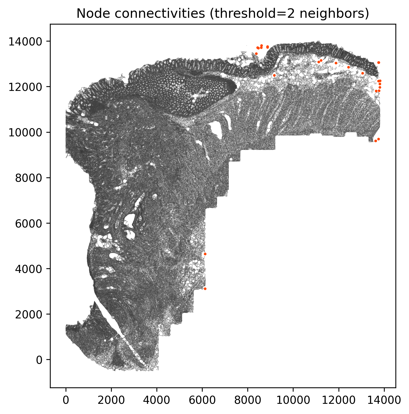
@fig-novae-connectivities confirms that a radius of 100 µm produces relatively few
isolated cells. If there were many isolated cells within regions, we might consider increasing
the radius.
```{r}
#| label: fig-novae-connectivities
#| message: false
#| warning: false
#| echo: false
#| fig.width: 8
#| fig.height: 7
#| fig-cap: "Cells with low connectivity (in red). "
#| eval: true
render(file.path(analysis_asset_dir, "domains"), "connectivity_plot.png",
dom_dir, overwrite = TRUE)
```
If you want to fine-tune the model based on your current data, you can run
the `fine_tune` method like so.
```{python}
#| label: novae-2
#| eval: false
#| code-summary: "Python Code"
#| message: false
#| warning: false
#| code-fold: show
import time
start_time = time.time() # Record the start time
model1.fine_tune(adata, max_epochs=50, logger=True, accelerator='cuda', num_workers=4) # <3>
end_time = time.time() # Record the end time
elapsed_time = end_time - start_time
print(f"Execution time: {elapsed_time:.4f} seconds")
novae_cells = adata.shape[0]
novae_fine_tune_seconds = elapsed_time
```
From the data and the model, we can compute the representations and assign cells
on of a varying number of domain levels. When saving domain levels, I like to increment
from one or two to a relatively high number and visualize on the tissue where domains
split. Let's save the model in case we ever want
to use it later and plot the domain hierarchy.
```{python}
#| label: novae-3
#| eval: false
#| code-summary: "Python Code"
#| message: false
#| warning: false
#| code-fold: show
start_time = time.time()
model1.compute_representations(adata, zero_shot=False, accelerator='cuda', num_workers=4) # <4>
end_time = time.time()
elapsed_time = end_time - start_time
print(f"Execution time: {elapsed_time:.4f} seconds")
novae_compute_representations_seconds = elapsed_time
for i in range(1, 12):
model1.assign_domains(adata, i)
model1_dir = os.path.join(dom_dir, "novae_model_one")
model1.save_pretrained(save_directory=model1_dir)
dh = model1.plot_domains_hierarchy()
plt.savefig(os.path.join(dom_dir, "novae_model1_hierarchy.png"), dpi=300, bbox_inches='tight')
plt.close()
adata.write_h5ad(
os.path.join(analysis_dir, "anndata-3-novae.h5ad"),
compression=hdf5plugin.FILTERS["zstd"],
compression_opts=hdf5plugin.Zstd(clevel=5).filter_options
)
```
1. If you are computing on CPU instead of GPU, accelerator should be set to 'cpu'.
```{r}
#| label: save-benchmarks
#| eval: false
#| code-summary: "R Code"
#| message: false
#| warning: false
#| code-fold: show
results_list[['novae_cells']] = py$novae_cells
results_list[['novae_fine_tune_seconds']] = py$novae_fine_tune_seconds
results_list[['novae_compute_representations_seconds']] = py$novae_compute_representations_seconds
saveRDS(results_list, results_list_file)
```
If you find that running the above code in CPU-only mode takes a long time and
you have GPUs available with cuda configured, I recommend trying `accelerator='cuda'`.
For this dataset with `r round(as.numeric(results_list[['novae_cells']]))` cells using
a single L4 GPU, it took `r round(as.numeric(results_list[['novae_fine_tune_seconds']])/60)`
minutes to run the fine tuning procedure and
`r round(as.numeric(results_list[['novae_compute_representations_seconds']])/60)` minutes
to compute representations.
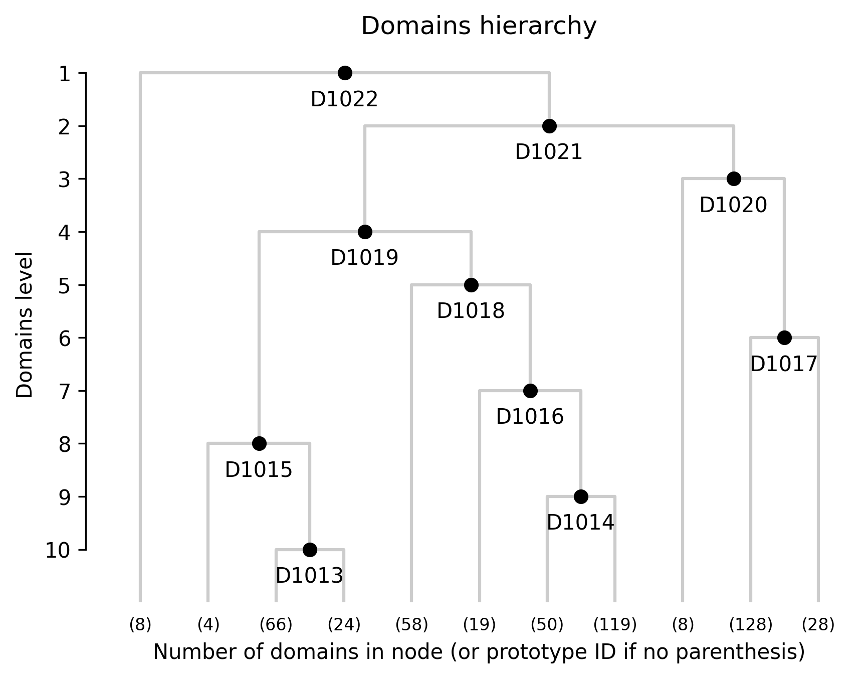
## Model Visuals
We assigned 11 domain levels. @fig-novae-model-1-hierarchy shows
the hierarchical relationship between them.
```{r}
#| label: fig-novae-model-1-hierarchy
#| message: false
#| warning: false
#| echo: false
#| fig.width: 8
#| fig.height: 7
#| fig-cap: "Hierarchical relationships among novae domains."
#| eval: true
render(file.path(analysis_asset_dir, "domains"), "novae_model1_hierarchy.png",
dom_dir, overwrite = TRUE)
```
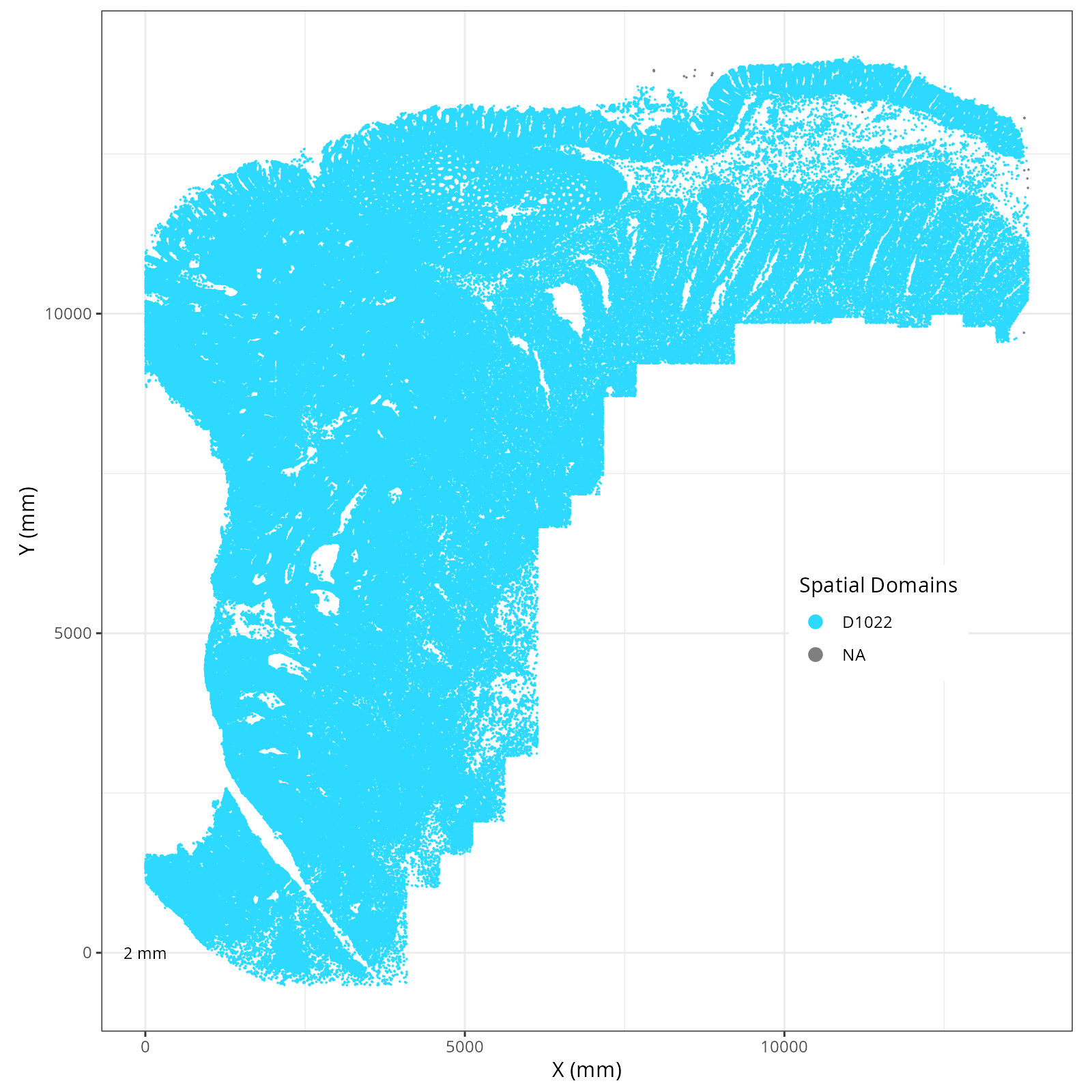
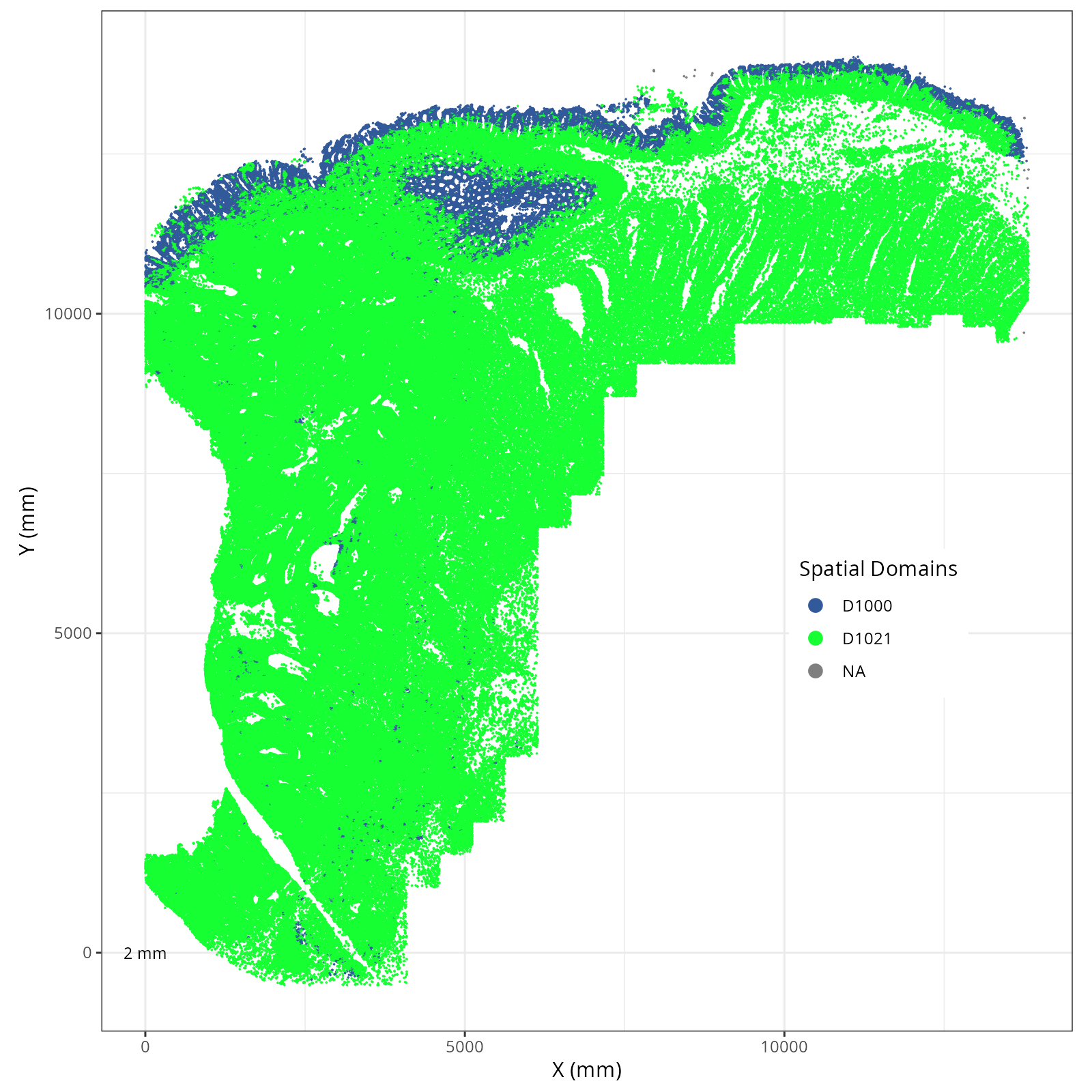
Plot these novae clusters in XY and UMAP space. As with @sec-processing, we'll make
use of the `plotDots` function after defining colors.
```{r}
#| label: novae-plots-1
#| eval: false
#| code-summary: "R Code"
#| code-fold: show
df <- py$adata$obs %>%
  select(starts_with("novae_domains_"))

domain_names <- c()
for(i in 1:ncol(df)){
  pick <- which(colnames(df)==paste0('novae_domains_', i))
  print(pick)
  domain_names <- c(domain_names, sort(unique(as.character(df[,pick]))))
}
domain_names <- unique(domain_names)

set.seed(98103)
domain_colors <- sample(pals::alphabet2(length(domain_names)))
names(domain_colors) <- domain_names
results_list[['novae_model_1_domain_names']] <- names(domain_colors)
results_list[['novae_model_1_domain_colors']] <- as.character(domain_colors)
saveRDS(results_list, results_list_file)
```
```{r}
#| label: novae-plots-2
#| eval: false
#| code-summary: "R Code"
#| code-fold: true
source("./helpers.R")
for(prefix in colnames(df)){
  plotDots(py$adata, color_by=prefix,
              plot_global = TRUE,
              facet_by_group = FALSE,
              additional_plot_parameters = list(
                  geom_point_params = list(
                    size=0.001
                  ),
                  scale_bar_params = list(
                    location = c(5, 0),
                    width = 2,
                    n = 3,
                    height = 0.1,
                    scale_colors = c("black", "grey30"),
                    label_nudge_y = -0.3
                  ),
                  directory = dom_dir,
                  fileType = "png",
                  dpi = 200,
                  width = 8,
                  height = 8,
                  prefix=prefix
                ),
              additional_ggplot_layers = list(
                theme_bw(),
                xlab("X (mm)"),
                ylab("Y (mm)"),
                coord_fixed(),
                scale_color_manual(values = domain_colors),
                theme(legend.position = c(0.8, 0.4)),
                guides(color = guide_legend(
                  title="Spatial Domains",
                  override.aes = list(size = 3) ) )
              )
              )
}
```
::: {.panel-tabset}
```{r}
#| output: asis
#| eval: true
#| code-fold: true
#| echo: false
fig_dir <- dom_dir
group_prefix <- "novae_domains_"
slide_id <- "S0"
xy_files <- Sys.glob(file.path(fig_dir,
paste0(group_prefix,
"*__spatial__", slide_id, "__plot*png")))
org_order <- as.numeric(gsub("novae_domains_", "", basename(sapply(strsplit(xy_files, split="__spatial"), "[[", 1L))))
xy_files <- xy_files[match(sort(org_order), org_order)]
res <- purrr::map_chr(xy_files, \(current_xy_file){
knitr::knit_child(text = c(
"### `r paste0('Domains: ', gsub('novae_domains_', '', basename(strsplit(current_xy_file, split='__spatial')[[1]][1])))`",
"",
"```{r eval=TRUE}",
"#| echo: false",
"knitr::include_graphics(current_xy_file)",
"```",
""
), envir = environment(), quiet = TRUE)
})
cat(res, sep = '\n')
```
:::
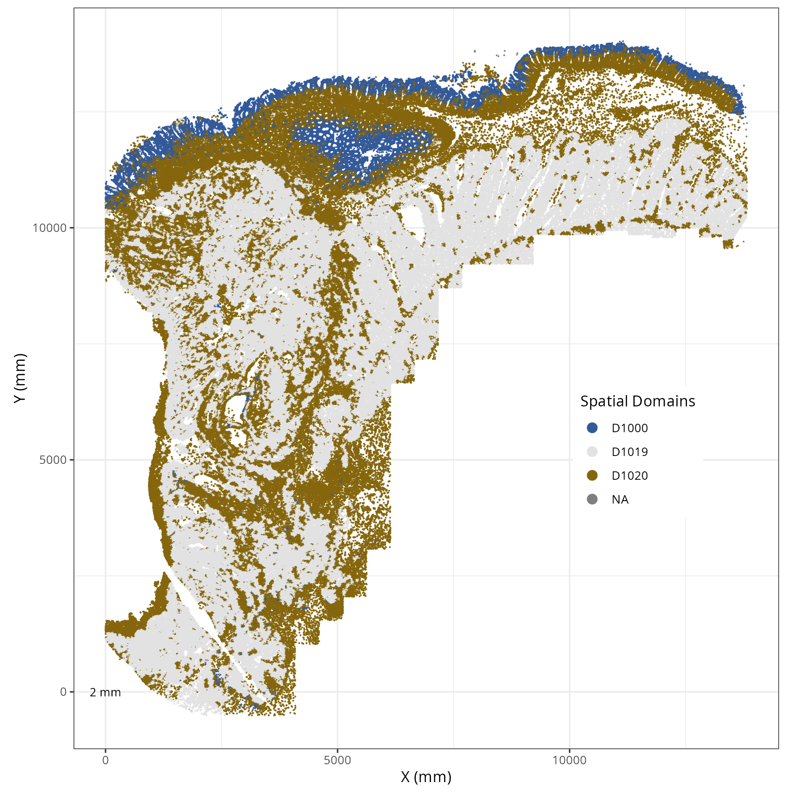
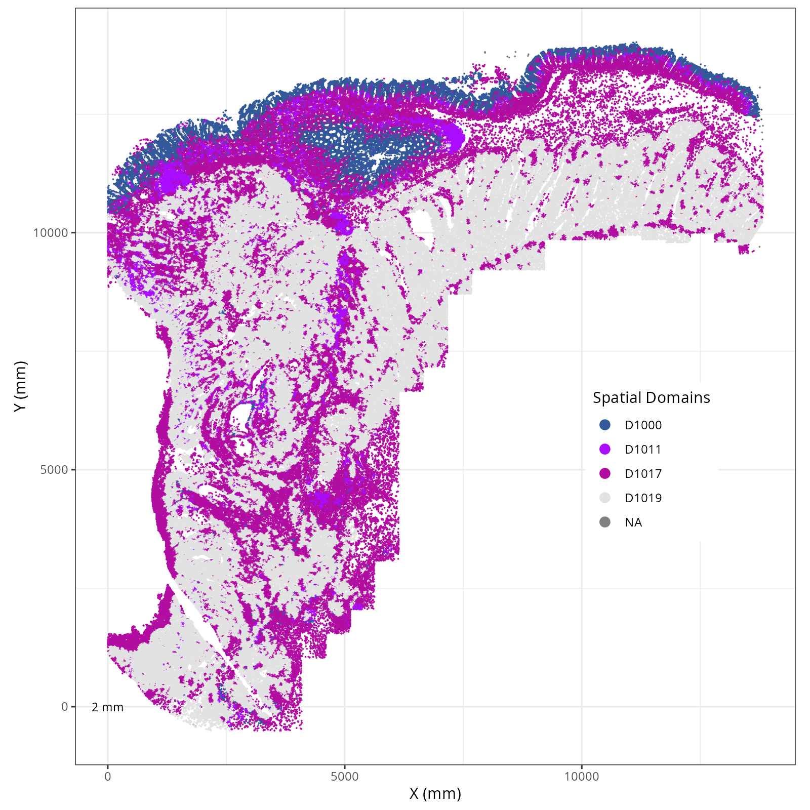
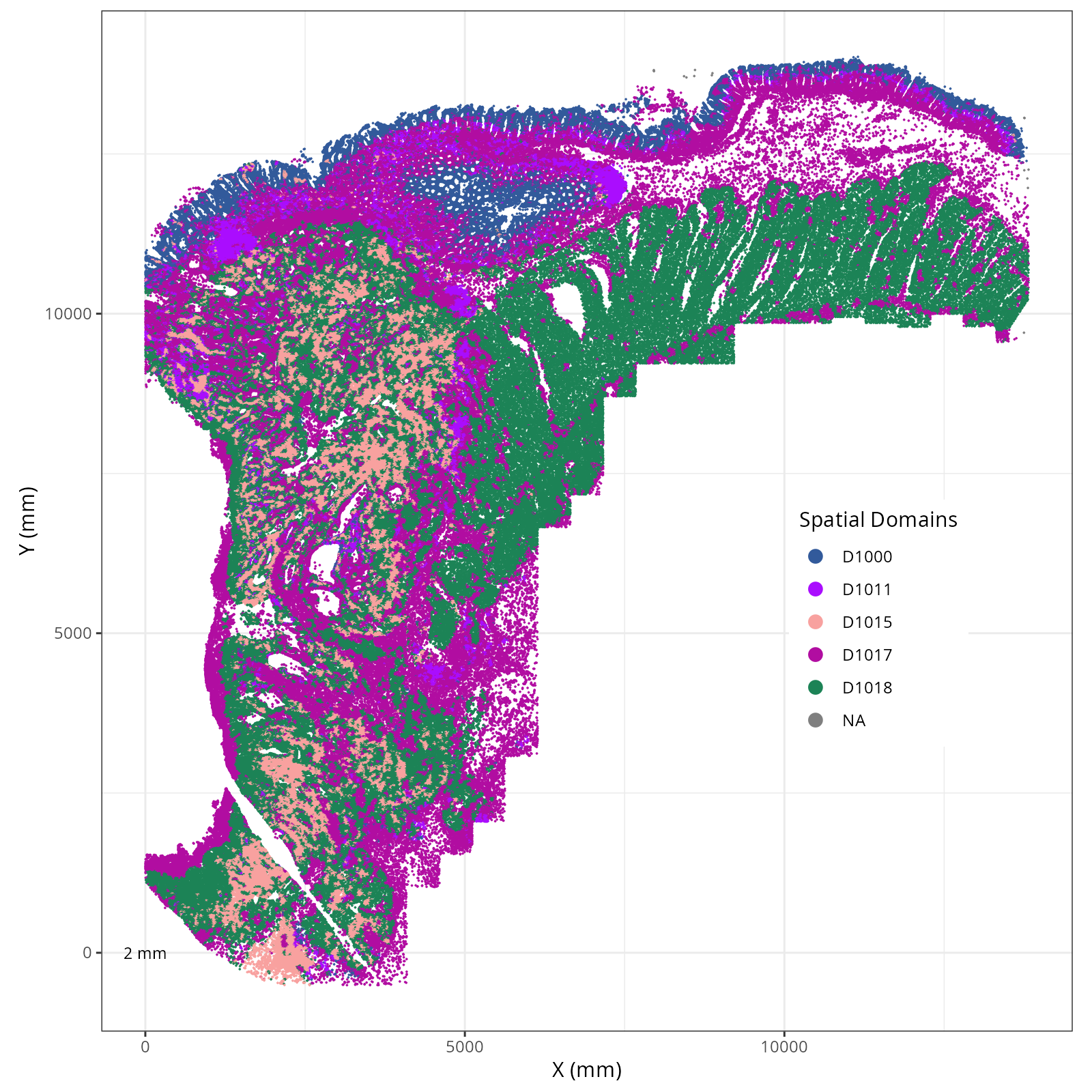
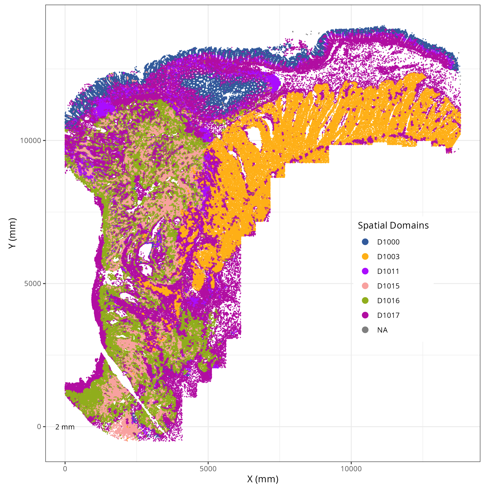
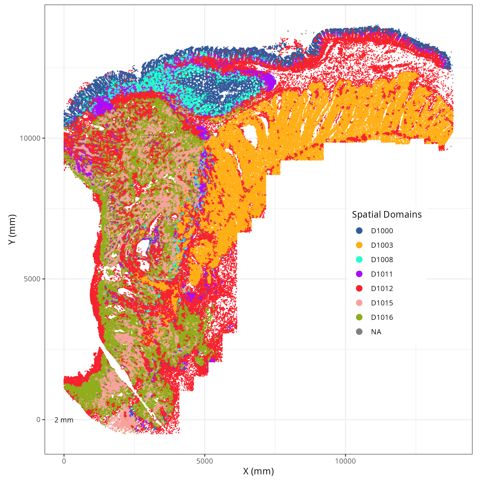
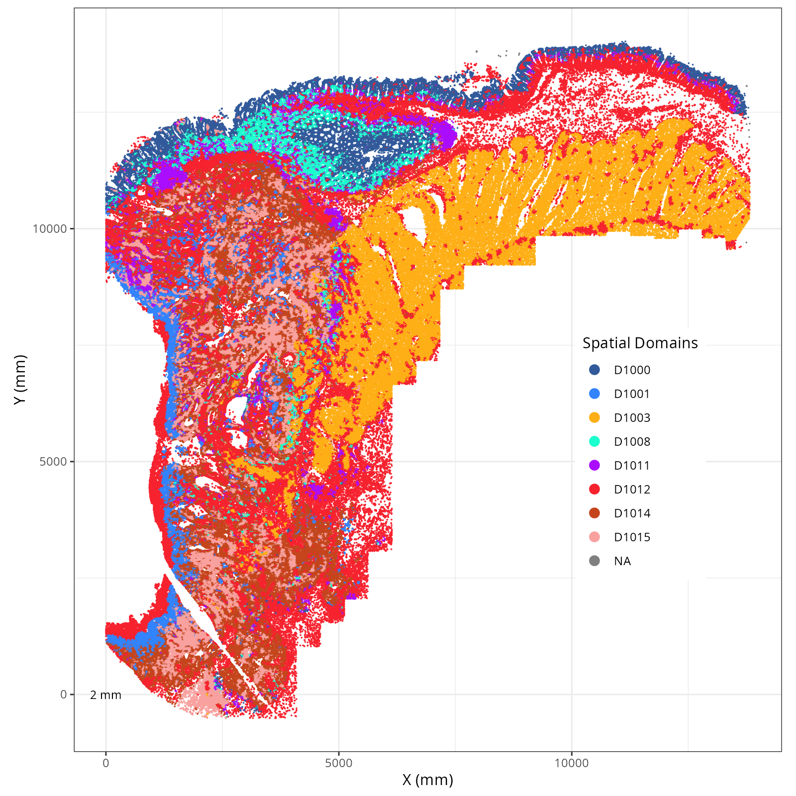
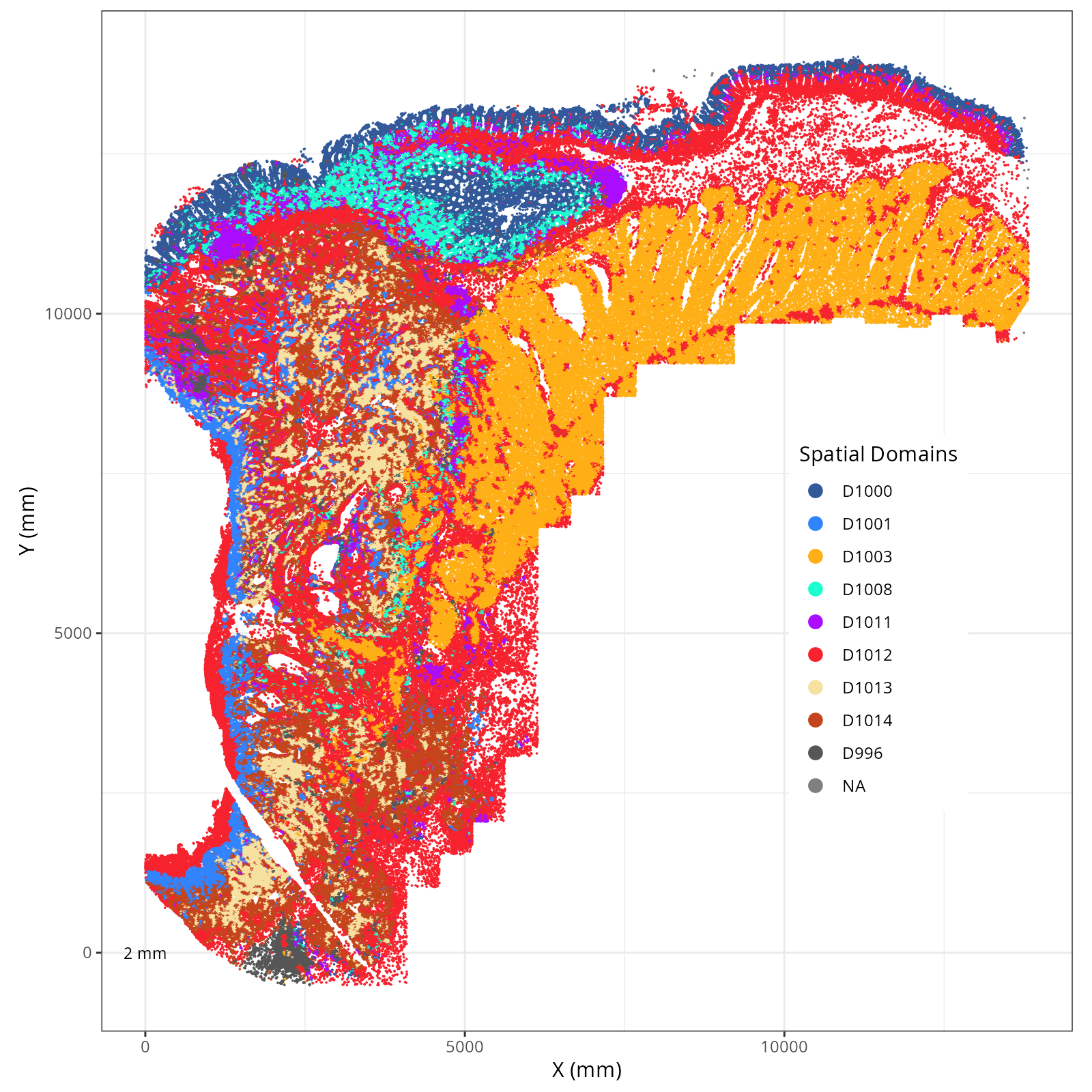
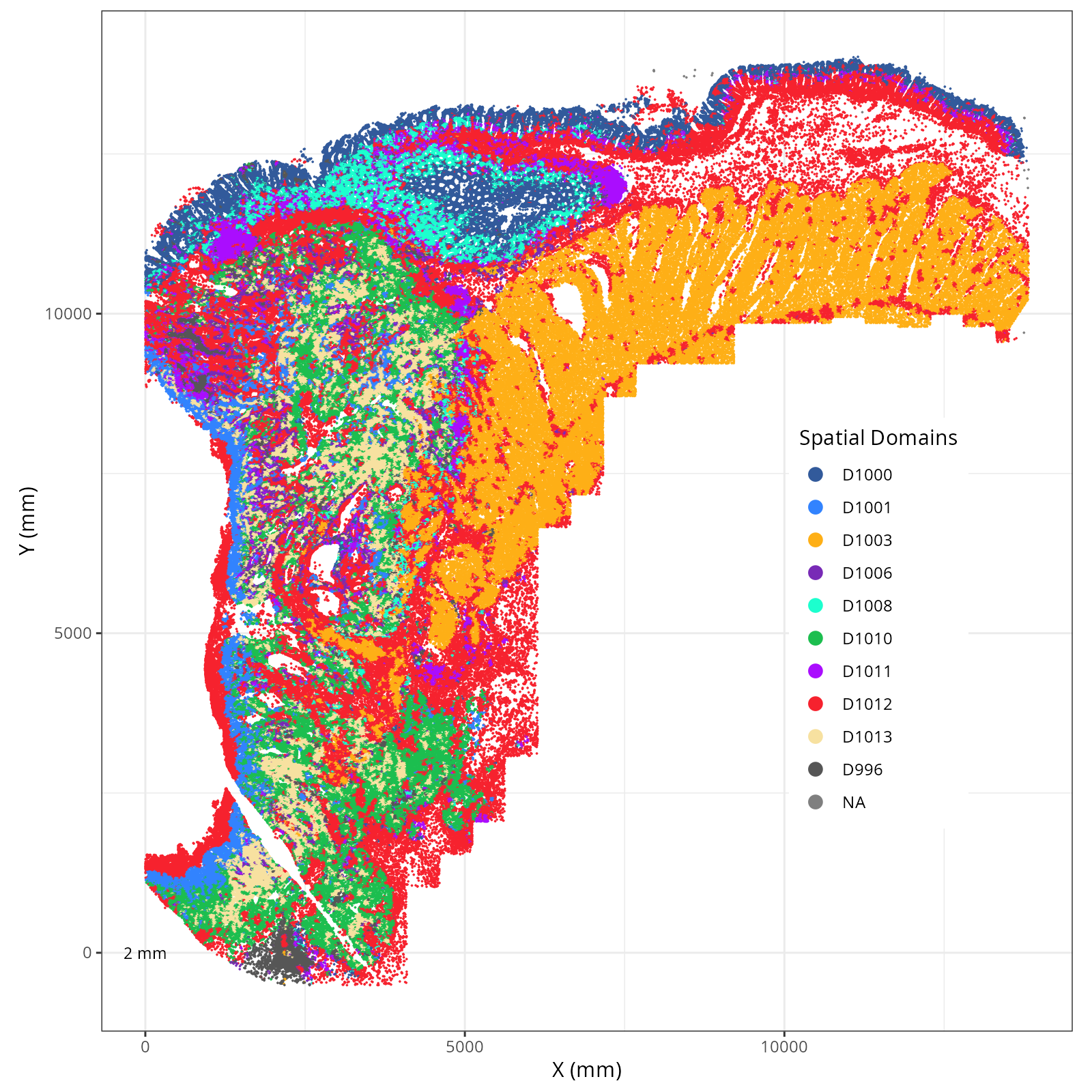
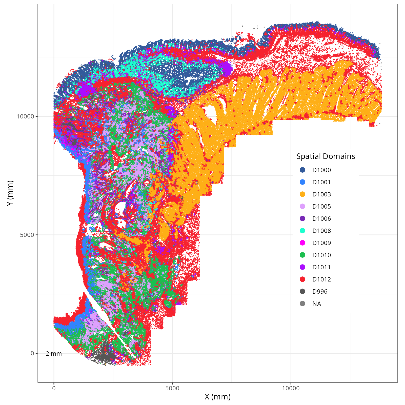
The choice of domain resolution depends on the types of biological questions that
are used. For example, if you wanted finer resolution of the micro-niches within the
epithelium (top part of the tissue, you may increase the number of domains). For
the purpose of this chapter, let's pick seven domains.
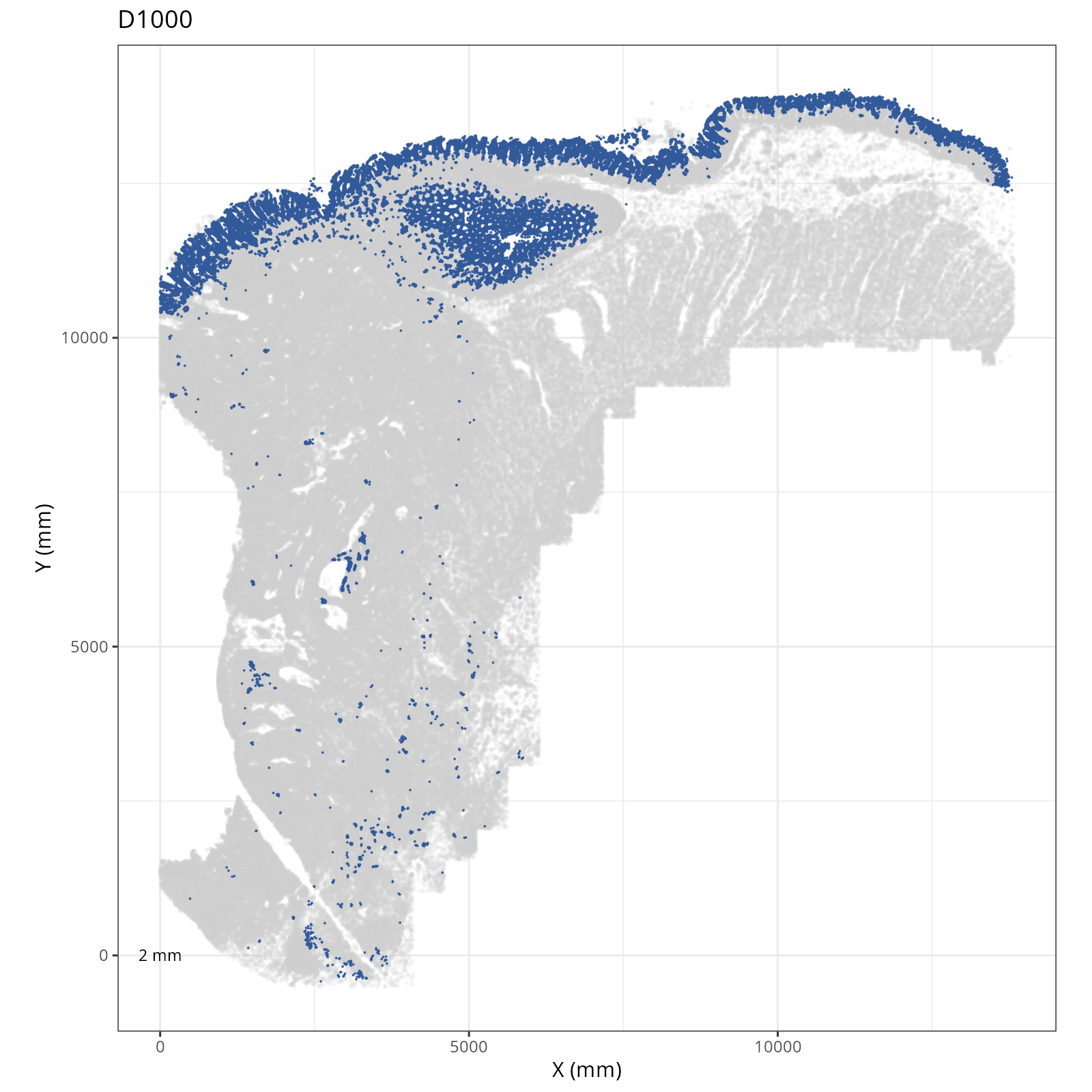
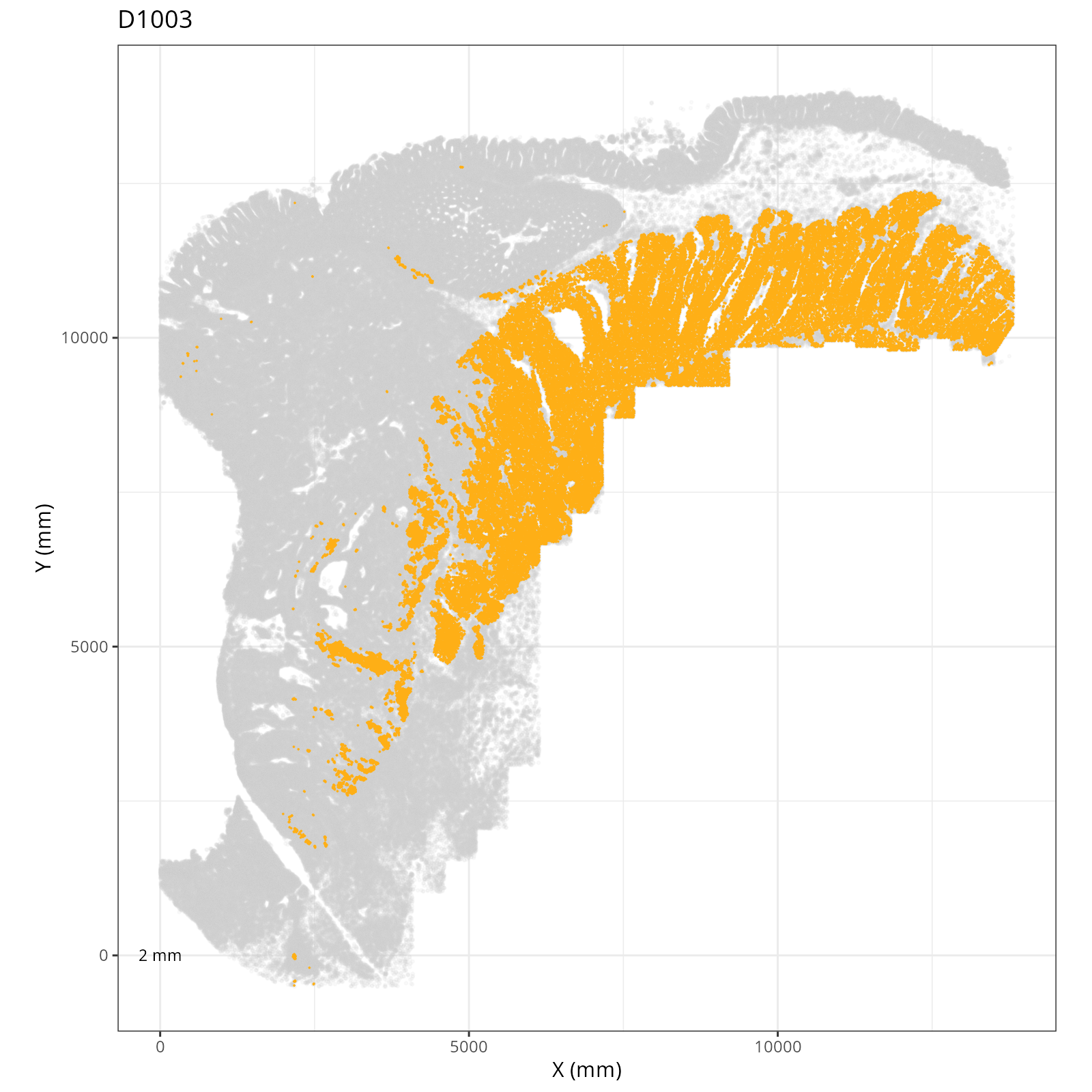
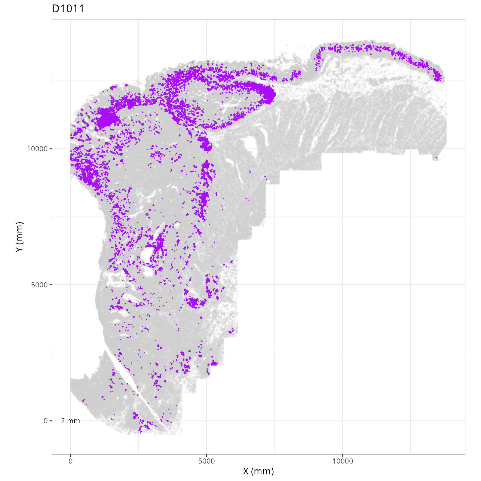
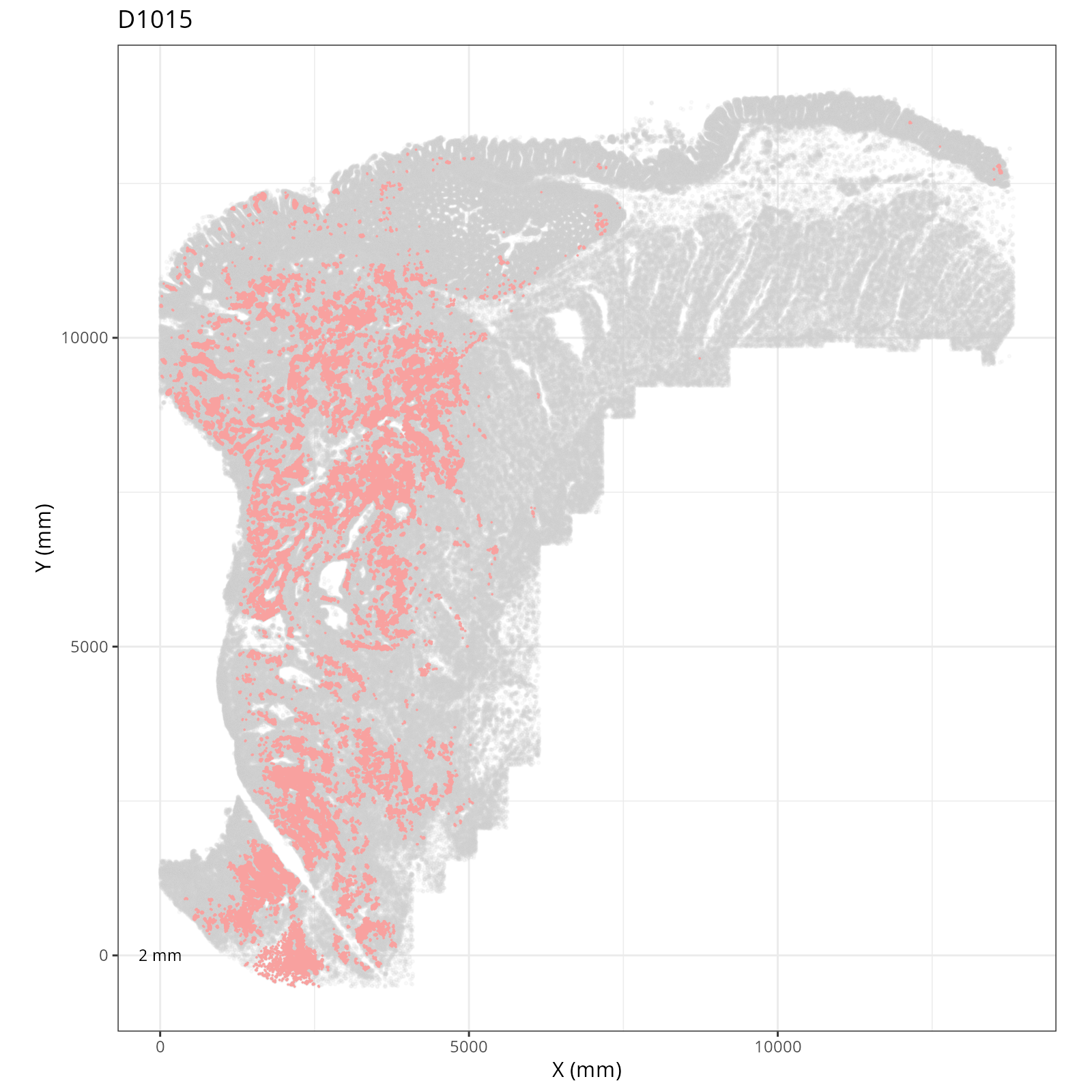
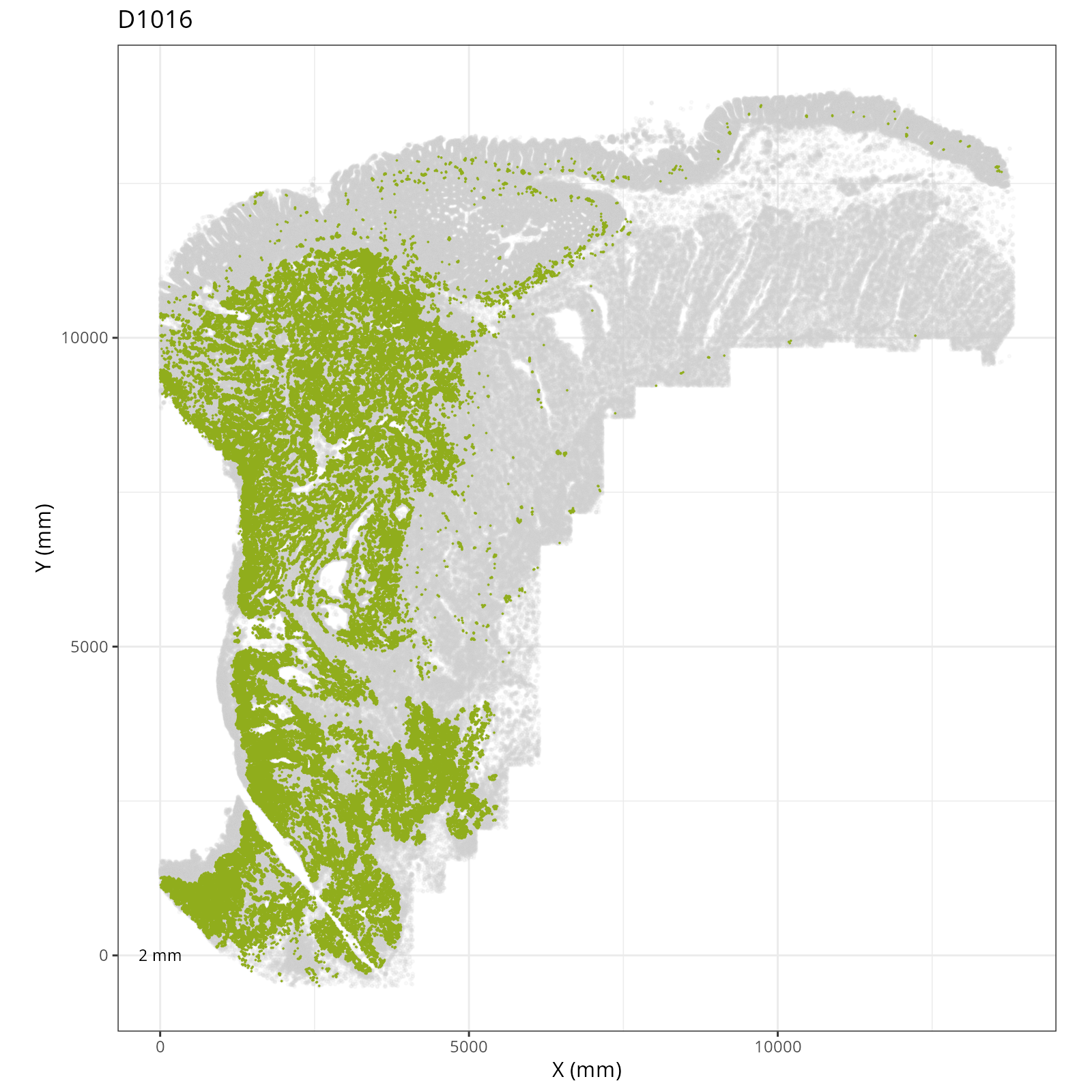
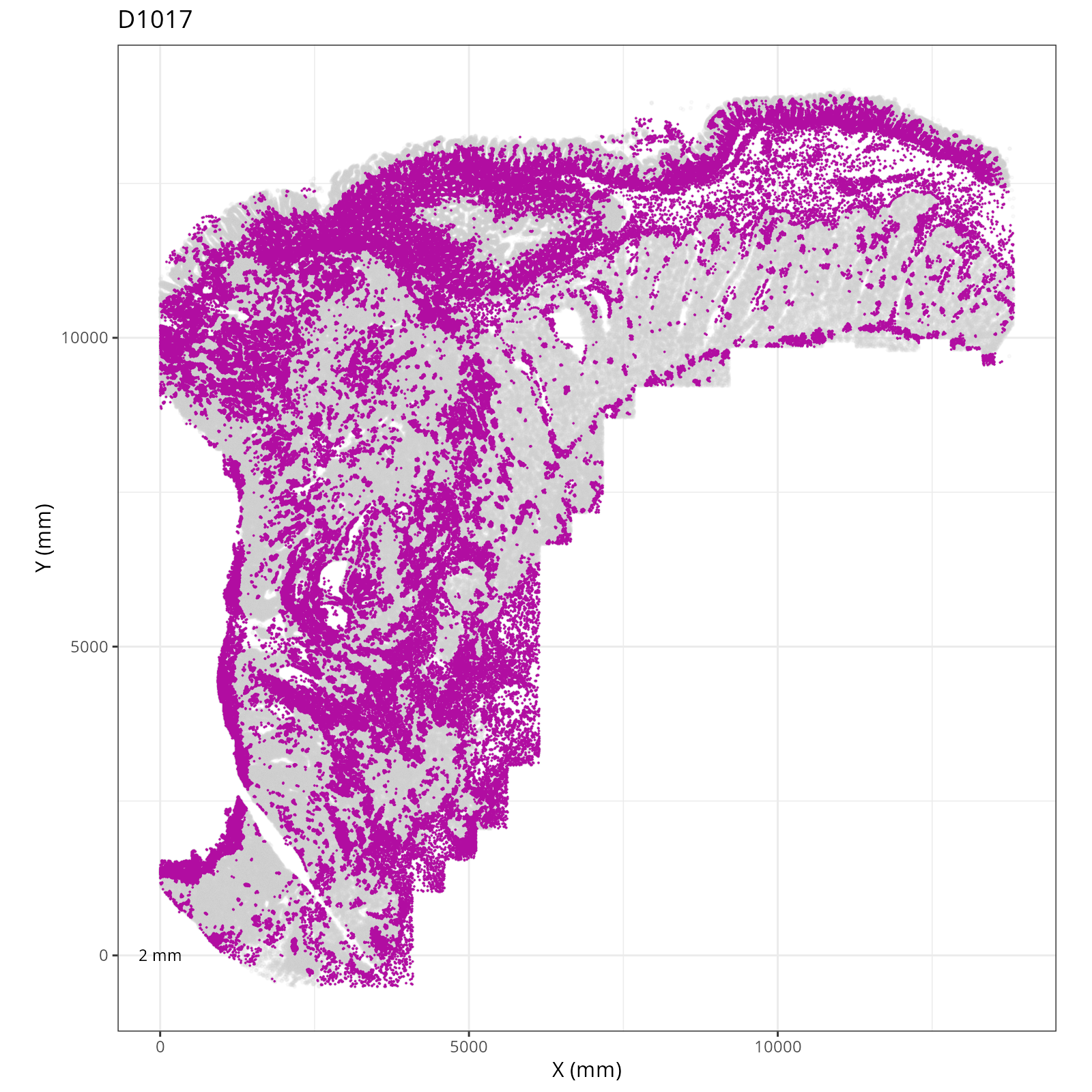
Focusing on six domain solution, plot individual XY plots to see the spatial
layout of each domain.
```{r}
#| label: novae-plots-3
#| eval: false
#| code-summary: "R Code"
#| code-fold: true
prefix <- "novae_domains_6"
plotDots(py$adata, color_by=prefix,
              plot_global = FALSE,
              facet_by_group = TRUE,
              additional_plot_parameters = list(
                  geom_point_params = list(
                    size=0.001
                  ),
                  scale_bar_params = list(
                    location = c(5, 0),
                    width = 2,
                    n = 3,
                    height = 0.1,
                    scale_colors = c("black", "grey30"),
                    label_nudge_y = -0.3
                  ),
                  directory = dom_dir,
                  fileType = "png",
                  dpi = 200,
                  width = 8,
                  height = 8,
                  prefix=prefix
                ),
              additional_ggplot_layers = list(
                theme_bw(),
                xlab("X (mm)"),
                ylab("Y (mm)"),
                coord_fixed(),
                scale_color_manual(values = domain_colors),
                theme(legend.position = c(0.8, 0.4)),
                guides(color = guide_legend(
                  title="Spatial Domains",
                  override.aes = list(size = 3) ) )
              )
              )
```
::: {.panel-tabset}
```{r}
#| output: asis
#| eval: true
#| code-fold: true
#| echo: false
# fig_dir <- file.path(analysis_asset_dir, "domains")
fig_dir <- dom_dir
group_prefix <- "novae_domains_"
slide_id <- "S0"
xy_files <- Sys.glob(file.path(fig_dir,
paste0(group_prefix,
"*__spatial__", slide_id, "__facet_*png")))
org_order <- as.numeric(gsub(".png", "", sapply(strsplit(xy_files, split="__facet_D"), "[[", 2)))
xy_files <- xy_files[match(sort(org_order), org_order)]
res <- purrr::map_chr(xy_files, \(current_xy_file){
knitr::knit_child(text = c(
"### `r paste0('Domain: ', gsub('.png', '', basename(strsplit(current_xy_file, split='__facet_')[[1]][2])))`",
"",
"```{r eval=TRUE}",
"#| echo: false",
"knitr::include_graphics(current_xy_file)",
"```",
""
), envir = environment(), quiet = TRUE)
})
cat(res, sep = '\n')
```
:::
## Conclusions
Now that we have the spatial domain assignments, the next step is to assign
functional names to these assignments. To aid in this effort, we'll first look at the composition
of cell types within these domains which is the topic of the next chapter.