2 Data Wrangling

source("./preamble.R")
reticulate::source_python("./preamble.py")
analysis_dir <- file.path(getwd(), "analysis_results")
input_dir <- file.path(analysis_dir, "input_files")
output_dir <- file.path(analysis_dir, "output_files")
analysis_asset_dir <- "./assets/analysis_results"
qc_dir <- file.path(output_dir, "output_files")
if(!dir.exists(qc_dir)){
  dir.create(qc_dir, recursive = TRUE)
}
results_list_file = file.path(analysis_dir, "results_list.rds")
if(!file.exists(results_list_file)){
  results_list <- list()
  saveRDS(results_list, results_list_file)
} else {
  results_list <- readRDS(results_list_file)  
}

1

This puts select images into the projects assets directory in enhance portability.

No data analysis journey can truly begin without first converting something and our task for this chapter is simple: take the flat files that are exported from AtoMx SIP into a usable format. That format is primarily python’s anndata format but, interestingly enough, we’ll take advantage of R’s data.table¹ package to efficiently read in the expression matrix file. I find this is much faster than reading in the expression matrix into pandas.

Alternative Approach

While this chapter focusing on converting the flat files into anndata format, it skips over other types of data that we can convert and use – such as the imaging data. Both Squidpy² and SpatialData³ offer ways to include composite images[^these are single images per FOV that combine the various IF channels together] into anndata objects. One limitation of these approaches – at the time of writing – is that they treat each FOV separately making it difficult to view results when you working with several hundred FOVs. For a tutorial on how to visualize the per-channel images across the entire sample with Napari, see this Scratch Space Blog.
In addition to processing and analyzing with python, R offers ways to analyze CosMx SMI data using packages like Seurat⁴. For an example on how to use Seurat for visualization, see Claire William’s Blog post and other vignettes.

Split the expression data into targets, negatives, and system controls. Read in the metadata and add columns that represent the slide position in micrometers.

tmp_dir <- "./tmp_dir"
dir.create(tmp_dir, showWarnings = FALSE)
flat_file_dir <- file.path(input_dir, "Run_b8806732_S2_Colon")
expression_dt <- data.table::fread(
  file.path(flat_file_dir, "S0_exprMat_file.csv.gz"),
  tmpdir = tmp_dir)

colnames(expression_dt)[which(colnames(expression_dt) == "cell_ID")] <- 'cell'
expression_dt <- expression_dt %>% arrange(fov, cell)
expression_dt <- expression_dt %>% mutate('cell_ID' = paste0("c_1_", fov, "_", cell))
cell_ids_vector_r <- expression_dt$cell_ID

all_feature_names <- setdiff(names(expression_dt), c("fov", "cell_ID", "cell"))

neg_indices_r <- which(startsWith(all_feature_names, "Negative") | startsWith(all_feature_names, "NegPr"))
sys_indices_r <- which(startsWith(all_feature_names, "System") | startsWith(all_feature_names, "False"))
gene_indices_r <- which(!startsWith(all_feature_names, "Negative") &
                          !startsWith(all_feature_names, "System") &
                          !startsWith(all_feature_names, "NegPr") &
                          !startsWith(all_feature_names, "False"))

neg_probe_names_vector_r <- all_feature_names[neg_indices_r]
sys_probe_names_vector_r <- all_feature_names[sys_indices_r]
gene_probe_cols <- all_feature_names[gene_indices_r]

neg_mat_r <- as.matrix(expression_dt[, ..neg_probe_names_vector_r])
sys_mat_r <- as.matrix(expression_dt[, ..sys_probe_names_vector_r])
gene_mat_r <- as.matrix(expression_dt[, ..gene_probe_cols])

meta <- data.table::fread(file.path(flat_file_dir, "S0_metadata_file.csv.gz"))

meta$tmp <- meta$cell_ID
meta$cell_ID <- meta$cell_id
meta$cell_id <- meta$tmp
meta$tmp <- NULL

meta <- meta %>% arrange(fov, cell_id)
um_per_px = 0.1203
meta$x_slide_mm <- um_per_px*meta$CenterX_global_px/1e3
meta$y_slide_mm <- um_per_px*meta$CenterY_global_px/1e3

if(nrow(meta) != nrow(gene_mat_r)){
  stop("Error. Check file inputs.")
}

1

My EC2 instance only has 100 GBs of storage. Setting it to a mounted drive without such restriction avoids low disk space warnings or complications.

2

This includes targets, negatives, and system controls

3

Keep dense. Avoid passing sparse matrices from/to R/python via reticulate

4

Conversion: 0.1203 µm per pixel

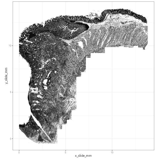
While the matrix and metadata information do not contain cell segmentation detail, it’s always a good idea to plot the cells in space to ensure they match our expected orientation.

p <- ggplot(data=meta) +
  geom_point(
    aes(x=x_slide_mm, y=y_slide_mm),
    size=0.001, alpha=0.1) + 
  coord_fixed() + theme_bw()

ggsave(filename = file.path(qc_dir, "xy_cells_initial_lowres.png"), p,
       width=8, height=8, dpi=80, type = 'cairo')
ggsave(filename = file.path(qc_dir, "xy_cells_initial_highres.png"), p,
       width=8, height=8, dpi=400, type = 'cairo')

1

I tend to plot lower-resolution versions of pngs to make the Quarto book light weight.

Figure 2.1 confirms the expected orientation and alignment from the flat files.

render(file.path(analysis_asset_dir, 'qc'), "xy_cells_initial_lowres.png", source_parent_folder=qc_dir)

Figure 2.1: Spatial oreientation of cells.

With that confirmation, create the initial anndata object. Specifically, we’ll start with dense¹ matrices of expression, system controls (i.e., “false codes”), and negative probes, and add these into the X elment and into obsm, respectively. We’ll place the metadata into the obs and we’ll also create a matrix of (X, Y) coordinates into their own obsm.

When analyzing interactively I switch between R and python blocks explicitly with reticulate::reply_python() to enter python and type exit() to return back to R.

filename = os.path.join(r.analysis_dir, "anndata-0-initial.h5ad")

if not os.path.exists(filename):
  # 1 Initial construction
  adata = ad.AnnData(
    X=r.gene_mat_r,
    obsm={'counts_neg': sp.sparse.csr_matrix(r.neg_mat_r), 'counts_sys': sp.sparse.csr_matrix(r.sys_mat_r)},
    obs=r.meta, 
    var=pd.DataFrame(index=r.gene_probe_cols),
  )
  adata.X = sp.sparse.csr_matrix(adata.X)
  adata.uns['neg_col_names'] = r.neg_probe_names_vector_r
  adata.uns['sys_col_names'] = r.sys_probe_names_vector_r
  
  # 2. add coordinates in the 'spatial' obsm
  coordinates = adata.obs[['x_slide_mm', 'y_slide_mm']].to_numpy()
  adata.obsm['spatial'] = coordinates
  
  # 3. Save object to disk
  adata.write_h5ad(
      filename,
      compression=hdf5plugin.FILTERS["zstd"],
      compression_opts=hdf5plugin.Zstd(clevel=5).filter_options
  )

1

Some packages expect the xy coordinates as a numpy array in obsm.

And that’s it! Our data have been converted into anndata format and now we’re ready to assess the quality.

1.

Barrett, T. et al. Data.table: Extension of ‘Data.frame‘. (2025).

2.

Palla, G. et al. Squidpy: A scalable framework for spatial omics analysis. Nat. Methods 19, 171–178 (2022).

3.

Marconato, L. et al. SpatialData: An open and universal data framework for spatial omics. Nat. Methods 22, 58–62 (2025).

4.

Hao, Y. et al. Dictionary learning for integrative, multimodal and scalable single-cell analysis. Nat. Biotechnol. 42, 293–304 (2024).

---

1. I generally avoid handing off sparse matrices from R to python and vice versa and since the data were dense to begin with (i.e., it was a CSV file), we’ll make it sparse in with python.