Here we propose an updated pipeline for basic CosMx® analysis in R, from data loading through cell typing. This workflow applies to all our RNA assays. Also see the companion posts on exploratory data analysis and confirmatory analysis with differential expression testing. A complete analysis will typically begin with the pre-processing described here, use exploratory analyses to generate hypotheses, then conclude by using differential expression analysis to test those hypotheses.
This code assumes a whole study can be fit into your compute environment’s memory. For very large studies, see our upcoming vignette on the topic.
This post is exclusively in R. Many steps have easy python analogs, but some, like the HieraType immune cell typing algorithm and the FOV QC functions, only have R implementations.
When your data is too large to fit into memory – and this can happen with just a few slides of WTX data – At this point, we recommend the below workflow, which we will demonstrate in a separate vignette in early 2026:
Obtain a subsample of the larger study. This could be FOVs chosen at random from all the tissues in the study, or just the first couple slides to come off the instrument.
Use this subsample to fix a basic pre-processing pipeline. Importantly, this pipeline has to be applicable to new samples: their data has to be projected onto the same dimension-reduced embedding, and their cell typing has to map to the cell typing of the subsample.
Apply the above pre-processing pipeline separately to each tissue/slide in the study.
Define an additional “hypothesis testing” pipeline, also to be applied separately to each tissue. This pipeline will compute whatever summary statistics you’re interested in, e.g. DE results, cell type abundance, LR interaction scores.
Perform meta-analysis of every tissues’ summary statistics together. E.g. contrast DE results or cell type abundances across responders and non-responders.
Custom subset analyses: you may also have to load in custom subsets of the data for analysis, e.g. just the macrophages from every tissue.
2 Loading flat files
First we’ll load the packages we need. Importantly, we’ll load “Matrix”, which handles sparse matrices. When a matrix has mainly zeroes, which is generally the case for single cell data, storing it in sparse matrix format has huge memory savings. Given the size of CosMx data, it is vital to be memory-efficient.
Code
# necessary librarieslibrary(data.table) # for more memory efficient data frameslibrary(Matrix) # for sparse matrices like our counts matrixlibrary(ggplot2)library(InSituCor) # devtools::install_github("https://github.com/Nanostring-Biostats/InSituCor")library(HieraType) # remotes::install_github("Nanostring-Biostats/CosMx-Analysis-Scratch-Space", subdir = "_code/HieraType", ref = "Main")library(Seurat)library(viridis)
AtoMx flat file exports come with each slide packaged in its own directory. Our example here has one slide, titled “BreastCancer”; its contents look like this:
So we have 5 files: an expression matrix, cell metadata, cell polygons, a map of fov positions, and the (very large) transcript locations file from this analysis. This analysis will only use the expression matrix and metadata. As such, you could reasonably export only those files from AtoMx. For examples on how to use the cell polygons in plots, see this post.
Now we’ll load in the flat files and format as we want.
Trying to load an entire matrix into memory at once may cause out-of-memory issues for large files.
In the code below, we load the counts matrices in chunks.
* First, we’ll use data.table::fread function which can directly read gzipped files, and determine how many rows and columns we’re working with.
* Then, we’ll read each chunk of data in, and convert it to a low-memory sparse matrix format before moving onto the next chunk.
* At the end, we’ll combine our sparse matrices to create the full data matrix.
Note: we’ll store our count matrices with cells in rows and genes in columns. Many protocols arrange their count matrix the other way around, but our approach here will be more performant for most operations.
To begin, tell your script where to operate:
Code
## set up:# location of flat files:# (point to a directory containing one folder of flat files per slide)myflatfiledir <-"path_to_your_flat_files_folder/flatFiles"# where to write output:outdir <-"path_to_your_desired_output_location"# set up results directories for laterif(!dir.exists(paste0(outdir, "/results"))){dir.create(paste0(outdir, "/results"))}# directory to hold intermediate data filesif(!dir.exists(paste0(outdir, "/processed_data"))){dir.create(paste0(outdir, "/processed_data"))}setwd(outdir)
The below code performs the loading and merging operations, producing 4 data objects:
A cell metadata matrix (cells x variables)
A counts matrix (cells x genes)
A matrix of cells’ xy positions (in mm)
(Optional) A negative control probe (“negprobe”) counts matrix (cells x negprobes)
(Optional) A SystemControl (“falsecode”) counts matrix (cells x falsecodes)
If given a flat files directory with multiple slides, it will seamlessly load and combine their data into a unified dataset.
Code
### source readFlatFiles:source("https://raw.githubusercontent.com/Nanostring-Biostats/CosMx-Analysis-Scratch-Space/Main/_code/vignette2/readFlatFiles.R")### automatically get slide names:slidenames <-dir(myflatfiledir)### load the flat files and return as distinct data objects:temp <-readFlatFiles(myflatfiledir, slidenames = slidenames, return_negprobes =FALSE, return_falsecodes =FALSE, offset_slides =TRUE) counts <- temp$counts; temp$counts <-NULLmetadata <- temp$metadata; temp$metadata <-NULLxy <- temp$xy; temp$xy <-NULLrm(temp)# checksstopifnot(identical(rownames(counts), metadata$cell_id))stopifnot(max(abs(Matrix::rowSums(counts) - metadata$nCount_RNA)) ==0)
Note that the above performs some well-advised modifications to the metadata:
Removes the “fov” column, which has duplicate values over multiple slides (e.g. any two slides will each have a fov 1). Replace it with the “FOV” column, which appends a slide identifier to FOV IDs so that each FOV has a unique id.
Removes the “cell_ID” column, which also can have duplicate values across slides, and retain the duplicate-free column “cell_id”.
For convenience, extracts cells’ xy positions as a separate data object, and recasts them from pixel-scale to mm-scale.
Adds the mean negprobe counts to the metadata (the metadata has the sum of the negprobes already, but since negprobe counts vary across panels it’s worth recording this value now so we won’t have to remember our negprobe number later.)
Finally, we save these data objects as .RDS files. These files are smaller on disk (they benefit from more compression than flat files do), and they’re faster to read back into R.
Important
Please note that these files hold intermediate results for convenience during analysis; they are not official file formats supported by BSB.
Code
# save data in R-friendly form:saveRDS(counts, file =paste0(outdir, "/processed_data/counts_unfiltered.RDS"))saveRDS(metadata, file =paste0(outdir, "/processed_data/metadata_unfiltered.RDS"))saveRDS(xy, file =paste0(outdir, "/processed_data/xy_unfiltered.RDS"))
Now we have data in 3 locations:
The RDS files we just created
The flat files we began with
The original data on AtoMx SIP
This is unnecessary duplication, and since CosMx data is so large, storing extra copies can incur real cost. There are two feasible approaches:
Once you’ve finished your analysis, delete all the large .RDS files created during it. They can always be regenerated by re-running the analysis scripts. If you are computing on the cloud, re-running does incur some compute costs, but these are minor compared to the cost of indefinitely storing large files.
Once you’ve confirmed this data loading script has run successfully, you can safely delete the flat files - you won’t be using them again. If you do need to go back to them, they’ll be on AtoMx, ready to be downloaded again: AtoMx acts as a persistent, authoritative source of unmodified data.
3 Customizing the tissues’ spatial arrangements
To show multiple slides in the same spatial plot, or just to produce spatial plots without a lot of extraneous white space, we often have to shift around tissues’ and/or FOVs’ xy positions. (We of course will preserve the relative xy positions of any cells we plan to analyze together spatially.) Below are some tools and code chunks for facilitating these operations, some borrowed from this post.
The basic operations of customized xy layouts are as follows:
First, for multi-slide studies, adjust the slides’ xy positions so they don’t overlap. This function is called within our flat file reader, but you can call it again to customize how slides are tiled.
Code
# source the tiling function:source("https://raw.githubusercontent.com/Nanostring-Biostats/CosMx-Analysis-Scratch-Space/Main/_code/vignette2/utils/readFlatFiles.R")# define new xy positions in which multiple slides no longer overlap each other:xy <-condenseTissues(xy = xy, tissue = metadata$Run_Tissue_name, tissueorder =NULL, # optional, specify the order tissues are tiled inbuffer =1, # space between tissueswidthheightratio =4/3) # desired shape of final xy locations
Second, break your cells into spatially contiguous groups (which may be separate tissues from one slide, or merely discontinuous FOV blocks from the same tissue). This can be done manually, as in the below chunk where we select cells in a selected xy range:
Code
# select a group of cells based on cutoffs in xy:xrange <-c(3.4, 5.2)yrange <-c(6.1, 8)thisgroup <- ((xy[, 1] > xrange[1]) & (xy[, 1] < xrange[2])) & ((xy[, 2] > yrange[1]) & (xy[, 2] < yrange[2]))
Or, we can automatically group contiguous FOVs using the dbscan algorithm:
Code
# cells within eps range of each other will be grouped together. # Set eps appropriately to link sufficiently close FOVs and separate sufficiently distant FOVs. # An FOV's width is about 1 mm. cellgroups <- dbscan::dbscan(xy, minPts =1, eps =1)$cluster# confirm the grouping is as desired:plot(xy, pch =16, cex =0.1, asp =1, col =sample(colors())[as.numeric(as.factor(cellgroups))])
Third, we rearrange groups. We can move groups manually:
Code
# shift a group of cells to the right:xy[thisgroup, 1] <- xy[thisgroup, 1] +1# or up:xy[thisgroup, 2] <- xy[thisgroup, 2] +5
…or we can move them automatically using the same condenseTissues function we used above:
Code
xy <-condenseTissues(xy = xy, tissue = cellgroups, tissueorder =NULL, # optional, specify the order tissues are tiled inbuffer =1, # space between tissueswidthheightratio =4/3) # desired shape of final xy locations
4 QC
QC of CosMx data is mostly straightforward. Technical effects can be complex, but they manifest in limited ways:
Many individual cells can have low signal
Segmentation errors can create “cells” with bad data
Sporadic FOVs can have low signal
Sporadic FOVs can have distorted / outlier expression profiles
Our workflow will create then add to flag, a vector marking cells flagged for one reason or another. When we’re done, we’ll delete everything we’ve flagged. (The full original data will remain on AtoMx, so this step is not as drastic as it seems. For smaller studies it could still be reasonable to hold on to the pre-QC .RDS files.)
4.1 Per-cell QC:
First, we’ll apply a threshold on cells’ total counts. Our defaults are fairly permissive; it would be reasonable to double them in datasets where you can do so without throwing out too many cells.
Code
# require sufficient counts per cell hist(log2(metadata$nCount_RNA), breaks =100, xlab ="Log2 counts per cell", ylab ="N cells", main ="")## cut off the low tail: # recommendations:# - 1000plex: 20 (permissive) or 50 (conservative)# - 6000plex: 50 (permissive) or 100 (conservative)# - WTX: 100 (permissive) or 200 (conservative)# - all panels: no more than 5% of cells (permissive) or 10% of cells (conservative)count_threshold <-min(200, quantile(metadata$nCount_RNA, 0.10)) # apply threshold, but don't flag >10% of cellsabline(v =log2(count_threshold), col ="red")flag <- metadata$nCount_RNA < count_thresholdlegend("topleft", legend =paste0(round(mean(flag) *100, 1), "% rejected"))mean(flag)
Next we’ll throw out cells with excessively large areas. In most studies, these “cells” are the result of segmentation errors. This step typically removes very few cells.
Code
# what's the distribution of areas?hist(metadata$Area, breaks =100, main ="", xlab ="Cell area (pixels)")# based on the above, set a threshold well out into the tail:area_threshold <-30000abline(v = area_threshold, col ="red")legend("topright", legend =paste0(round(mean(metadata$Area > area_threshold) *100, 2), "% rejected"))# flag cells based on area:flag <- flag | (metadata$Area > area_threshold)mean(flag)
Note
Note: some tissues do have very large cells, e.g. purkinje cells in the brain or cardiomyocytes in the heart. You’ll likely want to skip the area filter in those studies.
To check for segmentation errors, consider our R package FastReseg, which uses transcript positions to flag cells with likely segmentation errors, then remove or reassign transcripts assigned to the wrong cells. We also advise examining the segmentation results in AtoMx’s tissue viewer; studies will occasionally need to be re-segmented under a different set of parameters.
4.2 FOV QC
We check FOVs for two indicators of artifacts: diminished total counts, and biased gene expression profiles. Procedures for both these checks, along with a detailed discussion, can be found in a method described here.
To summarize briefly: for each “bit” in our barcodes (e.g. red in reporter cycle 8), we look for FOVs where genes using the bit are underexpressed. We also look for FOVs where total expression is suppressed.
Below we’ll run our FOV QC code and examine its results:
Code
## preparing resources:# source the FOV QC tool:source("https://raw.githubusercontent.com/Nanostring-Biostats/CosMx-Analysis-Scratch-Space/Main/_code/FOV%20QC/FOV%20QC%20utils.R")# load necessary information for the QC tool: the gene to barcode map:allbarcodes <-readRDS(url("https://github.com/Nanostring-Biostats/CosMx-Analysis-Scratch-Space/raw/Main/_code/FOV%20QC/barcodes_by_panel.RDS"))names(allbarcodes)# get the barcodes for the panel we want:barcodemap <- allbarcodes$Hs_WTX # <------- choose the right map for your panelhead(barcodemap)## run the method:fovqcresult <-runFOVQC(counts = counts, xy = xy, fov = metadata$FOV, barcodemap = barcodemap) saveRDS(fovqcresult, file =paste0(outdir, "/processed_data/fovqcresult.RDS"))# map of flagged FOVs:mapFlaggedFOVs(fovqcresult)# list FOVs flagged for any reason, for loss of signal, for bias:fovqcresult$flaggedfovsfovqcresult$flaggedfovs_fortotalcountsfovqcresult$flaggedfovs_forbias# flag cells in flagged FOVs:flag[is.element(metadata$FOV, fovqcresult$flaggedfovs)] <-TRUE# plot the result:FOVSignalLossSpatialPlot(fovqcresult)
We don’t have any flagged FOVs in this study. For examples of studies with more flagged FOVs, see the FOV QC post and this older vignette. The FOV signal loss plot above does show variation in signal strength, but that variation appears to track spatially smooth biology, likely contours of tumor glands, rather than sharp FOV boundaries.
4.3 Descriptive QC plots
In addition to the above per-cell flags, it can be worth plotting some QC metrics atop the space of your tissues. The purpose of these plots is to become aware of possible technical effects that might explain any artifacts you discover later in analysis. In the vast majority of studies, these plots will not require any action from you.
First, plot total counts over space:
Code
## plot total counts over space:par(mar =c(0,0,0,0))plot(xy, pch =16, cex =0.1, asp =1, col =viridis_pal(option ="B")(101)[round(1+100* (log2(pmin(pmax(metadata$nCount_RNA, 10), 5000)) -log2(10)) /log2(5000)) ])legendvals <-c(10, 100, 1000, 5000)legend("bottomright", pch =16, col =c("white", viridis_pal(option ="B")(101)[round(1+100* (log2(legendvals) -log2(10)) /log2(5000))]),legend =c("Total counts:", legendvals))
We see ample variability in total counts over space, but it all appears biological, not technical, with the exception of some FOV edge effects in which cells partially captured at some FOV edges have suppressed counts.
We also like to plot background over space. Because negative control counts are so sparse at the level of single cells, we plot spatially smoothed background, i.e. we color each cell by the mean background over its 50 nearest neighbors. To isolate background tendency from overall signal strength, we also normalize our background (negprobe) counts to each cells’ total RNA counts.
We see some regions of elevated background. No immediate action is needed, but by becoming aware of these isolated technical effects we’ll be armed to interpret any strange results driven by them. High local background often occurs in regions of necrosis.
Finally, we plot flagged cells in space:
Code
# plot flagged cells in space:par(mar =c(0,0,0,0))plot(xy, pch =16, cex =0.1, asp =1, col =c("grey80", "red")[1+ flag])
We can see flagged cells clustered in ducts/vessels/gaps in the tissue. Again, no action is needed, but we should keep this in mind while we interpret results.
4.4 Removing flagged cells
As our final QC step, we remove flagged cells and save the filtered data for downstream analysis:
Code
# save data with flagged cells removedcounts <- counts[!flag, ]metadata <- metadata[!flag, ]xy <- xy[!flag, ]# save filtered data objects, to be used in the remainder of the analysissaveRDS(counts, file =paste0(outdir, "/processed_data/counts.RDS"))saveRDS(metadata, file =paste0(outdir, "/processed_data/metadata.RDS"))saveRDS(xy, file =paste0(outdir, "/processed_data/xy.RDS"))
5 Normalization
We typically normalize each cell’s expression profile to its total counts. The below code does this efficiently. In fact, given the size of the matrix and the speed of this calculation, there is no need to save a normalized data object; it’s cheaper to re-compute it than to store it.
Code
# normalize counts matrix using efficient sparse matrix calls:# (recall our counts matrix has cells in rows and genes in columns)scale_row <-mean(metadata$nCount_RNA) / metadata$nCount_RNAnorm <- countsnorm@x <- norm@x * scale_row[norm@i +1L]
Note that no steps in this workflow actually use the normalized data, although the dimension reduction step performs its own normalization under the hood. Normalized data will be useful in later analyses, e.g. for plotting expression over space or running differential expression.
We do not generally use a log1p transformation. Pearson residuals have nice properties, but they produce a dense matrix, which is too memory-intensive for most studies. (See below for how we nonetheless get PC’s based on Pearson residuals.)
6 Dimension reduction
Here we demonstrate an important improvement in dimension reduction for large studies. The single cell analysis world has long used Pearson residuals to normalize & transform their data prior to running PCA; these residuals scale count data to better balance the information available in each cell / gene. However, Pearson residuals are dense, meaning we cannot encode them with a sparse matrix, making them computationally intractable for larger datasets. To benefit from Pearson residuals without taxing our compute instances, we have developed a method of calculating the principal components of a Pearson residual matrix without ever having to store the entire matrix. A full description is here. We demonstrate this function below.
We’ll start by identifying highly variable genes. In this section we’ll take advantage of some of the functions in the Seurat ecosystem.
Code
# make a seurat object:library(Seurat)seu <- Seurat::CreateSeuratObject(counts = Matrix::t(counts),meta.data = metadata)# find HVG's:# recommend nfeatures = 3000 for WTX, 2000 for 6k panel, and using all features for 1k panelsseu <- Seurat::FindVariableFeatures(seu, nfeatures =3000) hvgs <-setdiff(seu@assays$RNA@meta.data$var.features, NA)saveRDS(hvgs, file =paste0(outdir, "/processed_data/hvgs.RDS"))
Next we run our Pearson residual-based PCA algorithm. You can install it with this command:
Code
# install the sparse pearson PCA package:remotes::install_github("Nanostring-Biostats/CosMx-Analysis-Scratch-Space",subdir ="_code/scPearsonPCA", ref ="Main")
The algorithm runs in two versions: standard, and batch-aware. The batch-aware version allows for gene frequencies that vary across some categorical batch variable like tissue or slide.
Note the code saving the output. This lets us re-run the script without waiting for long algorithms to reprocess. However, this particular routine runs fast enough, and generates a large enough data object, that it would also be reasonable to recalculate rather than store its output.
## get PCs based on Pearson residuals:# version without batch adjustment:if (TRUE) { genefreq <- scPearsonPCA::gene_frequency(Matrix::t(counts)) ## gene frequency (across all cells) pcaobj <- scPearsonPCA::sparse_quasipoisson_pca_seurat(x = Matrix::t(counts[, hvgs]),totalcounts = metadata$nCount_RNA,grate = genefreq[hvgs],scale.max =10, ## PC's reflect clipping pearson residuals > 10 SDs above the mean pearson residualdo.scale =TRUE, ## PC's reflect as if pearson residuals for each gene were scaled to have standard deviation=1do.center =TRUE## PC's reflect as if pearson residuals for each gene were centered to have mean=0 )saveRDS(pcaobj, file =paste0(outdir, "/processed_data/pcaobj.RDS")) } else { pcaobj <-readRDS(paste0(outdir, "/processed_data/pcaobj.RDS"))}
Code
# In this example code we assume the metadata has a column "patient" that we wish to treat as a possible batch effectif (TRUE) { genefreq_batch <- scPearsonPCA::gene_frequency(x = Matrix::t(counts),obs = metadata[,.(cell_id, patient)],cellid_colname ="cell_id",batch_variable ="patient") pcaobj <-sparse_quasipoisson_pca_seurat_batch( Matrix::t(counts[, hvgs]),totalcounts = metadata$nCount_RNA,grate = genefreq_batch[hvgs,],obs = metadata[,.(cell_id, patient)],batch_variable ="patient",cellid_colname ="cell_id",scale.max =10,do.scale =TRUE,do.center =TRUE )saveRDS(pcaobj, file =paste0(outdir, "/processed_data/pcaobj.RDS"))} else { pcaobj <-readRDS(paste0(outdir, "/processed_data/pcaobj.RDS"))}
Next we’ll obtain a UMAP projection from those PCs:
Code
## run UMAP:if (TRUE) { umapobj <- scPearsonPCA::make_umap(pcaobj)# save the full object: the umap connectivity graph will be useful later on:saveRDS(umapobj, file =paste0(outdir, "/processed_data/umapobj.RDS"))} else { umapobj <-readRDS(paste0(outdir, "/processed_data/umapobj.RDS"))}## plot the UMAP projection, coloring by total counts:par(mar =c(0,0,0,0))plot(umapobj$ump@cell.embeddings, pch =16, asp =1, cex =0.1,col = scales::alpha(viridis_pal(option ="B")(101)[round(1+100* (log2(pmin(pmax(metadata$nCount_RNA, 10), 5000)) -log2(10)) /log2(5000)) ], 0.05))legendvals <-c(10, 100, 1000, 5000)legend("topleft", pch =16, col =c("white", viridis_pal(option ="B")(101)[round(1+100* (log2(legendvals) -log2(10)) /log2(5000))]),legend =c("Total counts:", legendvals))
7 Cell typing
7.1 Unsupervised clustering
Here we demonstrate the most consistently successful approach to cell typing we have found. (Supervised cell typing with InSituType can also work quite well, but depends on a good reference marix.) First, we perform unsupervised clustering using a set of a few thousand highly variable genes (hvg’s). Second, we use the HieraType algorithm to obtain accurate immune cell classification, then overwrite our initial clustering results with HieraType’s calls wherever it finds immune cells. This approach is robust, and requires minimal configuration and re-running. Naming clusters used to be time-consuming, but we have found that the right prompts to a large language model (LLM), combined with rigorous oversight, minimize the burden of cluster naming. We will demonstrate two approaches to unsupervised clustering:
Louvain clustering, using PC’s derived from Pearson residuals of hvg’s.
InSituType’s unsupervised mode, run on hvg’s.
Of the above two methods, Louvain tends to be faster, while InSituType is easier to refine, and, more importantly, straightforward to project onto future datasets. (InSituType clusters come with mean expression profiles which can be used as input to InSituType’s supervised cell typing mode.)
Note: Here we run louvain clustering with a high resolution, intentionally over-clustering with the plan to condense afterwards. It’s often better to run with the default resolution (0.8) at first, then subcluster selected cell types afterwards. To sub-cluster a cell type, first filter out genes for which segmentation errors are likely to bias its profiles. Use smiDE::overlap_ratio_metric to do so. (smiDE is available on the scratch space.)
Code
# use Seurat to run Louvain clustering on the graph from our umap objectif (TRUE) { seu[["pearsongraph"]] <- Seurat::as.Graph(umapobj$grph) ## nearest neighbors / adjacency matrix used for unsupervised clusteringset.seed(0) seu <- Seurat::FindClusters(seu, graph ="pearsongraph", resolution =1.2) # choosing a high resolution with the plan to condense afterwards clust <- seu@meta.data$seurat_clusterssaveRDS(clust, file =paste0(outdir, "/processed_data/clust.RDS"))} else { clust <-readRDS(paste0(outdir, "/processed_data/clust.RDS"))}# save to metadatametadata$clust <- clustcellcols <-rep(c("#E41A1C", "#377EB8", "#4DAF4A", "#984EA3", "#FF7F00","#A65628", "#F781BF", "#999999", "#66C2A5", "#FC8D62","#8DA0CB", "#E78AC3", "#A6D854", "#FFD92F", "#E5C494","#B3B3B3", "#1B9E77", "#D95F02", "#7570B3", "#E7298A","#66A61E", "#E6AB02", "#A6761D", "#666666", "#A6CEE3","#1F78B4", "#B2DF8A", "#33A02C", "#FB9A99", "#E31A1C","#FDBF6F", "#FF7F00", "#CAB2D6", "#6A3D9A", "#FFFF99","#B15928", "#8DD3C7", "#FFFFB3", "#BEBADA", "#FB8072"), 3)[1:length(unique(clust))]# Quick xy and umap plots of clusters to confirm resolution looks right:plot(umapobj$ump@cell.embeddings, pch =16, asp =1, cex =0.1, col = scales::alpha(cellcols[as.numeric(as.factor(clust))], 0.05))plot(xy, pch =16, asp =1, cex =0.1, col = cellcols[as.numeric(as.factor(clust))])
Here we refer you to the InSituType vignette. Running in unsupervised mode is simplest, though supervised and semi-supervised modes can work well provided with good reference profiles.
A call to InSituType that would work with our setup here is:
Code
if (TRUE) {set.seed(0) unsup <-insitutype(x = counts[, hvgs], # only use HVG's. InSituType's computation time scales with the number of genes, so analyzing the full WTX panel is very slow. neg = metadata$negmean,assay_type ="RNA", reference_profiles =NULL,reference_sds =NULL,cohort =NULL, # see the InSituType docs for how to use this argument to incorporate spatial information into clusteringn_clusts =20,n_starts =5,max_iters =25 ) saveRDS(unsup, file =paste0(outdir, "/processed_data/unsup.RDS"))} else { unsup <-readRDS(paste0(outdir, "/processed_data/unsup.RDS"))}# save resultsmetadata$clust <- clust <- unsup$clust# Quick xy and umap plots of clusters to confirm resolution looks right:plot(umapobj$ump@cell.embeddings, pch =16, asp =1, cex =0.1, col = scales::alpha(cellcols[as.numeric(as.factor(clust))], 0.05))plot(xy, pch =16, asp =1, cex =0.1, col = cellcols[as.numeric(as.factor(clust))])
7.2 Naming clusters
Determining which cell type a cluster corresponds to is a complex exercise that should take into account:
The cluster’s marker genes
Its overall abundance
Its spatial locations
This can be onerous, but we can get a big jump start on this work by using large language models (LLM’s). Below, we’ll create a custom prompt asking a LLM to name your cluster. We have found LLM’s to do a very good (though not perfect) job of naming cell types given this information. After this step we’ll show how to QC your cell type assignments.
As a first step, we’ll derive marker genes for our clusters:
Code
if (TRUE) { markers <- HieraType::clusterwise_foldchange_metrics( Matrix::t(counts),metadata = metadata,cluster_column ="clust",cellid_column ="cell_id")saveRDS(markers, file ="processed_data/markers.RDS")} else { markers <-readRDS("processed_data/markers.RDS")}# get a more succinct list of markers: only the top N per cell type:# prioritize by fold change, but penalize low-expressers:markers$prioritystat <- (markers$cluster_expr +0.025) / (markers$clusterprime_expr +0.025)markersshort <-c()nperclust <-5for (name inunique(markers$cluster)) { inds <- markers$cluster == nameif (length(inds) >0) { markersshort <-c(markersshort, markers$gene[inds][order(markers$prioritystat[inds], decreasing =TRUE)[1:min(nperclust, sum(inds))]]) }}
In addition to data-derived marker genes, we’ll also look at a pre-defined list of well-known markers of broad cell types and lineages.
Code
# load general-purpose lineage and marker genes:source("https://raw.githubusercontent.com/Nanostring-Biostats/CosMx-Analysis-Scratch-Space/Main/_code/vignette2/lineage_and_marker_genes.R")# (loads the list "lineagegenes")# save both selected markers and lineage genes:allusefulmarkers <-intersect(colnames(counts), unique(c(unlist(lineagegenes), markersshort)))
Now that we have marker genes identified, we can proceed to crafting an LLM prompt:
Code
## describe your tissue here. mytissuetype <-"HER2+ breast cancer"# the preamble:prompt_preamble <-paste0("Please propose cell type names for the clusters I\'ve found in a CosMx study. This is data from a ", mytissuetype, ". ","Below are two tables. The first is each cell type\'s abundance in the dataset. ","The second is a table of mean expression levels of various marker genes and lineage-defining genes in each cluster. ","It\'s possible that some clusters could be closely-related cell types, or distinct states of the same cell type. Call that out when it\'s apparent. ","For each cluster, give me your best guess at its identity, and give me your justification. Let me know when you\'re uncertain. ","Then, give me R code defining a named vector called \'cluster_labels\' in which my cluster IDs are the names and the values are your proposed cell types. ","Don\'t hallucinate, and check your work three times. ")# info on cluster frequencies:prompt_frequencies <-paste0("The cluster frequencies are: ", paste0(paste0("cluster ", names(table(clust)), ":", table(clust)), collapse =", "))## give the LLM each cluster's mean expression profile over relevant genes:# obtain a matrix of the clusters' marker gene profiles:allusefulmarkers <-intersect(colnames(counts), unique(c(unlist(lineagegenes), markersshort)))meanexpression <- markers[, dcast(.SD, gene ~ cluster, value.var ="cluster_expr")]meanexpression <-as.matrix(meanexpression[, -1]) # drop gene colrownames(meanexpression) <- markers[, unique(gene)]meanexpression <- meanexpression[allusefulmarkers, ]# reduce to just lineage genes with decent expression (but keep de novo markers):isdenovo <-is.element(rownames(meanexpression), markersshort)meanexpression <- meanexpression[isdenovo |apply(meanexpression, 1, max) >0.2, ]prompt_profiles <-paste0("And here is a table of each cluster's mean expression of selected data- and biology-derived marker genes: ",paste(capture.output(write.table(round(meanexpression, 1), sep =",", row.names =TRUE, col.names =TRUE) ), collapse ="\n"))message(paste0(prompt_preamble, "\n", prompt_frequencies, "\n", prompt_profiles))# save old results for rewriting later on:unnamedclust <- clustunnamedmeanexpression <- meanexpression
This creates the below prompt, which can be copied into whichever LLM you prefer:
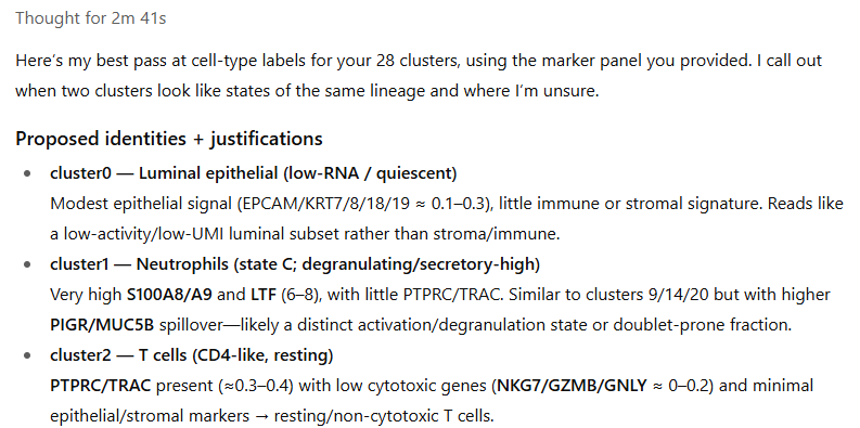
When this prompt was passed to ChatGPT5, it produced a writeup that looked like this:
… and more importantly, the below code ready to be copy-pasted into our analysis:
Code
cluster_labels <-c("0"="Luminal epithelial (low-RNA/quiescent)","1"="Neutrophils (state C, degranulating/secretory-high)","2"="T cells (CD4-like, resting)","3"="IFN-high epithelial (luminal, inflamed)","4"="Luminal epithelial (apocrine-leaning; state A)","5"="CAFs (matrix-rich fibroblasts)","6"="Antigen-presenting myeloid (cDC2 / moDC)","7"="Luminal epithelial (apocrine-high; state B)","8"="Luminal epithelial (apocrine-high; state C)","9"="Neutrophils (state B)","10"="Luminal epithelial (apocrine-secretory)","11"="Luminal epithelial (apocrine-high; state D)","12"="Luminal epithelial (apocrine-very-high; state E)","13"="Macrophages (APOE+/C1QA+ TAMs)","14"="Neutrophils (state A; S100A8/A9-max)","15"="Epithelial–neutrophil admixture (uncertain)","16"="CAFs (cycling)","17"="Endothelial (blood/lymphatic mix)","18"="Inflamed epithelial with myeloid shadow (uncertain)","19"="Pericytes / vascular SMC","20"="Luminal epithelial (mucociliary-like secretory)","21"="Cycling epithelial","22"="Luminal epithelial (baseline state)","23"="IFN-high epithelial (luminal, inflamed)","24"="Luminal epithelial (mucociliary-like secretory)","25"="Plasma cells","26"="Antigen-presenting cells (B/cDC; cycling, uncertain)","27"="Cytotoxic T / NK cells")# for now, just uncritically take the names. Clustering QC and possible renaming will come later.metadata$clust <- clust <- cluster_labels[as.character(unnamedclust)]colnames(meanexpression) <- cluster_labels[as.character(gsub("cluster", "", colnames(unnamedmeanexpression)))]
7.3 QC of clustering results
The LLM gave us a good guess at cluster names, but we still need to verify them. To assist in this process, we recommend looking at 4 outputs:
The LLM’s justifications for its calls
A heatmap of each cluster’s expression of key marker genes
The clusters’ distributions in space.
The clusters’ UMAP positions
The code below draws the key plots:
Code
# heatmap of marker genes - drawn tall so we can read all gene names:dev.off() # need to silence the current graphics device for a pheatmap pdf to render properlypdf(paste0(outdir, "/results/marker heatmap tall.pdf"), height =17, width =6)pheatmap::pheatmap(sweep(meanexpression, 1, pmax(0.1, apply(meanexpression, 1, max)), "/"),col =colorRampPalette(c("white", "darkblue"))(101),fontsize_row =6)dev.off()# umap positionspng("results/umap_by_cluster.png", width =16, height =16, units ="in", res =400)par(mar =c(0,0,0,0))plot(umapobj$ump@cell.embeddings, pch =16, asp =1, cex =0.1, col = scales::alpha(cellcols[as.numeric(as.factor(clust))], 0.05))legend("topleft", pch =16, legend =levels(as.factor(clust)), col = cellcols[1:length(levels(as.factor(clust)))])dev.off()# xy positions:for (name inunique(clust)) {png(paste0("results/cluster xy - ", make.names(name), ".png"), width =diff(range(xy[, 1])) *0.5, height =diff(range(xy[, 2])) *0.5,unit ="in", res =350)par(mar =c(0,0,0,0))plot(xy, pch =16, cex =0.1, col = scales::alpha(cellcols, 0.3)[as.numeric(as.factor(clust))], xlab ="", ylab ="", xaxt ="n", yaxt ="n")points(xy[clust == name, ], pch =16, cex =0.1, col ="black")legend("top", legend = name, bty ="n")dev.off()}
We obtain:
A .pdf heatmap of marker gene expression, stretched out to allow for scrutinizing gene names (not legible zoomed-out; meant to be explored via zooming and scrolling):
A .png showing each cluster in umap space, giving you another look at which clusters are similar to each other:
A .png for each cluster showing its positions in xy space (bold black points atop faded points for other clusters):
With these plots in hand, you should scrutinize the initial cluster names and correct as needed. Note that you can gloss over immune clusters: we’ll be overriding them later with the HieraType algorithm’s results.
To rename clusters, simply edit the cluster names in the definition of cluster_labels above, and re-run from that code block onward. This step can also be used to merge closely-related clusters by assigning multiple clusters the same name. In our case, we renamed three clusters of cancer cells that the LLM labeled as neutrophils (some of the classic neutrophil markers are also expressed by cancer cells).
Note
For tumor studies, additional techniques can help classify cancer cells:
Cancer cells tend to be extremely transcriptionally active. Clusters with high total counts per cell are usually cancer.
The scMalignantFinder algorithm promises to call cells as cancer vs. non-cancer. We have not tried it, but it seems promising.
For WTX studies, it’s possible to estimate cells’ copy number variants. Cells with clear CNV’s will usually be cancer. We have used insituCNV successfully. A newer method, ClonalScope, also looks promising.
8 Optimizing immune cell calling with the HieraType algorithm
8.1 Running HieraType
We created the HieraType algorithm to classify immune cells in a way that is informed by marker genes. We have found it to consistently outperform other algorithms in immune cell typing. Our standard approach now is to overwrite our initial clustering results with HieraType’s results whenever it calls an immune cell.
An important caveat: the HieraType workflow below was designed for solid tissues containing the typical infiltrating immune cell classes, i.e. everything you might expect to find in a solid tumor. For tissues with specialized immune cell types, e.g. progenitor cells, or immune-derived cancer cells, HieraType could still run but would need modifications to its marker genes / “pipeline” data object. See the HieraType package for a deeper read before setting that up.
Below, we run HieraType in two steps. In the first, we call broad cell types (e.g. epithelial, immune, …) then subclassify the immune cells (B, T, macrophage…)
Now we’ll use a simple marker heatmap to confirm HieraType worked as hoped:
Code
# pull out canonical ("index") markers:indexmarkers <-unique(c(unlist(pipeline_io_rna$markerslists$l2)[grepl("index_marker", names(unlist(pipeline_io_rna$markerslists$l2)))],unlist(HieraType::pipeline_tcell)[grepl("index_marker", names(unlist(HieraType::pipeline_tcell)))]))# make a marker heatmap for the hieratype immune cell calls:fcmetrics <- HieraType::clusterwise_foldchange_metrics(normed = Matrix::t(norm[, indexmarkers]),metadata =data.frame("cell_ID"=names(htclust), "hieratype_call"= htclust),cluster_column ="hieratype_call")hm_hier <- HieraType::marker_heatmap(fcmetrics, extras =NULL)print(hm_hier)
The above heatmap doesn’t show the strongest markers; it shows the most biologically-relevant markers. We can gain further confidence in our immune cell typing results looking at data-driven markers:
Code
fctbl_unsup <- HieraType::clusterwise_foldchange_metrics(normed = Matrix::t(norm),metadata =data.frame("cell_ID"=names(htclust), "hieratype_call"= htclust),cluster_column ="hieratype_call" )## make a marker heatmaphm_unsup <- HieraType::marker_heatmap(fctbl_unsup)print(hm_unsup)
8.2 Merging clustering and HieraType results
To finish our cell typing exercise, we now merge the Louvain and HieraType results. All cells called immune by HieraType will get HieraType labels. All other cells will retain their old labels, with one important exception: clusters that were overwhelmingly called immune by HieraType will be removed, and their cells will be assigned to whatever consensus cell type is most abundant in its nearest neighbors in expression space.
The code above provides a direct path through the basic preprocessing of CosMx data. With these results secured, you’re ready to proceed to the rewarding parts of data analysis: exploring your data and testing hypotheses. The next pages of this vignette discuss those topics. For exploratory analysis, differential expression, or any other further analysis, we recommend containing distinct analyses in standalone scripts, each beginning by loading the data we’ve prepared here:
Code
# load basic data:counts <-readRDS(paste0(outdir, "/processed_data/counts.RDS"))metadata <-readRDS(paste0(outdir, "/processed_data/metadata.RDS"))xy <-readRDS(paste0(outdir, "/processed_data/xy.RDS"))# get normalized data if desired:scale_row <-mean(metadata$nCount_RNA)/metadata$nCount_RNAnorm <- countsnorm@x <- norm@x * scale_row[norm@i +1L]# likely to be useful: compute nearest neighbors:neighbors <- InSituCor:::nearestNeighborGraph(xy[, 1], xy[, 2], N =50, subset = metadata$slide_ID)