Introduction to SpatialOmicsOverlay
Maddy Griswold, Megan Vandenberg, and Stephanie Zimmerman1
Source:vignettes/Introduction-to-SOO.Rmd
Introduction-to-SOO.RmdOverview
With GeoMx DSP, regions of interest (ROIs) are selected by the user
and then molecularly profiled within each ROI.
SpatialOmicsOverlay was specifically made to visualize and
analyze the free-handed nature of Region of Interest (ROI) selection in
a GeoMx experiment, and the immunofluorescence-guided segmentation
process. ROIs can be either profiled in the selected area (i.e.,
geometric profiling) or subdivided based on the visible morphology
markers into compartments and profiled separately (i.e., segmented
profiling). Probe counts collected from ROIs underly the genomic
expression signal. The overlay from the instrument is recreated in the R
environment, allowing for plotting overlays with data like ROI type or
gene expression.
This vignette demonstrates how to use OME-TIFF image files generated by the NanoString GeoMx ® Digital Spatial Profiler (DSP) instrument to enhance data visualization of your experiments. You will use as a case study one sample of mouse brain. We will be walking through how to plot the image, profiled regions, and their gene expression.
The SpatialOmicsOverlay package is now available through Bioconductor.
Note: Many of the later code chunks have
eval=FALSE–work through the vignette yourself to see the
images and plots!
About This Sample
The mouse brain sample in this vignette is one of four available from our Spatial Organ Atlas. While we will be looking at only one sample, any of the data from our freely-downloadable Spatial Organ Atlas samples would also suffice as an alternative.
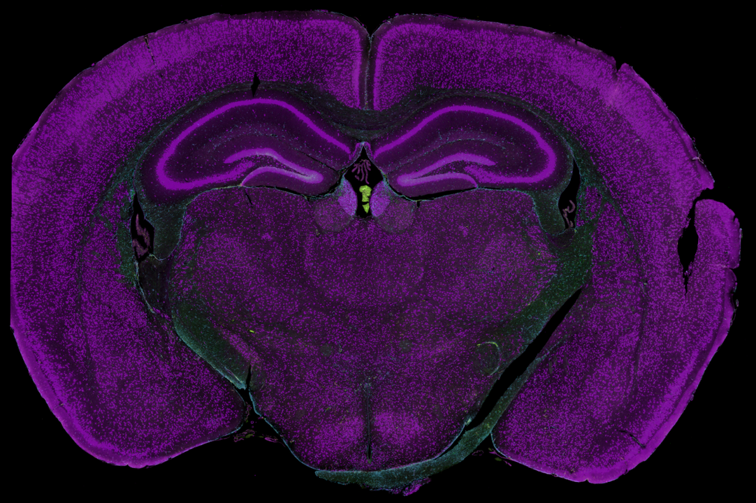
Mouse brain
This coronal section of formalin-fixed, paraffin-embedded (FFPE) adult mouse was visualized with antibodies to:
- NeuN (neuronal nuclei and perinuclear cytoplasm)
- GFAP (astrocytes)
- Iba1 (microglia)
- SYTO83 (nuclei)
This mouse brain features both geometric and segmented ROI profiling. For the segmented profiling, we mainly used NeuN as a morphology marker to segment the neuronal nuclei and neuropil regions on this sample:
- Neuronal nuclei - NeuN+
- Neuropil - NeuN-
Load Libraries
Note: We have occasionally observed this error when
running library(SpatialOmicsOverlay), which has
RBioFormats as a dependency:
Error: package or namespace load failed for 'SpatialOmicsOverlay':
  .onLoad failed in loadNamespace() for 'RBioFormats', details:
  call: jclassName(class, class.loader = class.loader)
  error: java.lang.ClassNotFoundException
We theorize this is due to the Dockerized RStudio warming
up and downloading the cached RBioFormats jar file, launching the JVM,
or other initiating processes. If you are encountering this error, we
recommend waiting several minutes between logging into RStudio and
running this vignette. We have also had success in repeatedly restarting
R (not RStudio) and running the Load Libraries chunk again.
If the issue persists, you may consider generating a new container from
the Docker image. Finally, it may be helpful to wait until the
RBioFormats cached jar file is fully in place before loading
SpatialOmicsOverlay; see the following code chunk.
# fn <- "~/.cache/R/RBioFormats/bioformats_package_6.12.0.jar"
# file.exists(fn, recursive =TRUE)
#
# if (file.exists(fn)) {
#   print(file.info(fn)$size)
#   if(file.info(fn)$size == 43081858) {
#     library(SpatialOmicsOverlay)
#   }
# }
library(rJava)
library(RBioFormats)
#> BioFormats library version 6.12.0
library(SpatialOmicsOverlay)
#> Registered S3 method overwritten by 'GGally':
#>   method from
#>   +.gg   ggplot2
library(GeomxTools)
#> Loading required package: Biobase
#> Loading required package: BiocGenerics
#>
#> Attaching package: 'BiocGenerics'
#> The following objects are masked from 'package:rJava':
#>
#>     anyDuplicated, duplicated, sort, unique
#> The following objects are masked from 'package:stats':
#>
#>     IQR, mad, sd, var, xtabs
#> The following objects are masked from 'package:base':
#>
#>     anyDuplicated, aperm, append, as.data.frame, basename, cbind,
#>     colnames, dirname, do.call, duplicated, eval, evalq, Filter, Find,
#>     get, grep, grepl, intersect, is.unsorted, lapply, Map, mapply,
#>     match, mget, order, paste, pmax, pmax.int, pmin, pmin.int,
#>     Position, rank, rbind, Reduce, rownames, sapply, setdiff, sort,
#>     table, tapply, union, unique, unsplit, which.max, which.min
#> Welcome to Bioconductor
#>
#>     Vignettes contain introductory material; view with
#>     'browseVignettes()'. To cite Bioconductor, see
#>     'citation("Biobase")', and for packages 'citation("pkgname")'.
#> Loading required package: NanoStringNCTools
#> Loading required package: S4Vectors
#> Loading required package: stats4
#>
#> Attaching package: 'S4Vectors'
#> The following object is masked from 'package:utils':
#>
#>     findMatches
#> The following objects are masked from 'package:base':
#>
#>     expand.grid, I, unname
#> Loading required package: ggplot2
Data Ingestion
Files needed:
- OME-TIFF from GeoMx instrument. (Other OME-TIFFs should work with custom parsing functions.)
- Lab Worksheet from instrument readout.
- Annotation file(s):
- Lab Worksheet
- GeomxSet Object (see GeomxTools and GeoMxWorkflows for more info)
- Annotations from DSPDA (DSP Data Analysis software)
In this example, we are downloading a TIFF image from AWS S3, but this variable is simply the file path to an OME-TIFF.
This function will be downloading a 13 GB file and will keep a 4 GB file in BiocFileCache. This download should take ~15 minutes, but you will only have to download once. Note this will download inside of the Docker image, but requires sufficient space on your device hosting the image.
tifFile <- downloadMouseBrainImage()
tifFile
#> [1] "/github/home/.cache/R/SpatialOmicsOverlay/6cbe7c583c_mu_brain_004.ome.tiff"
downloadMouseBrainImage() will download files, in this
workshop, to the
/home/rstudio/.cache/R/SpatialOmicsOverlay/ folder.
Reading in the SpatialOverlay object can be done with or without the image. We will start without the image, as that can be added later.
If outline = TRUE, only ROI outline points are saved.
This decreases memory needed and figure rendering time downstream. If
ANY ROIs are segmented in the study, outline will be FALSE. In this
particular example, there are segmented ROIs, so we set
outline = FALSE.
muBrainLW <- system.file("extdata", "muBrain_LabWorksheet.txt",
                        package = "SpatialOmicsOverlay")
muBrain <- readSpatialOverlay(ometiff = tifFile, annots = muBrainLW,
                             slideName = "4", image = FALSE,
                             saveFile = FALSE, outline = FALSE)
#> Extracting XML
#> Parsing XML - scan metadata
#> Parsing XML - overlay data
#> Warning in parseOverlayAttrs(omexml = xml, annots = annots, labworksheet = labWorksheet): Some AOIs do not match annotation file.
#> Not Matched: DSP-1012996073013-H-C01, DSP-1012996073013-H-C07, DSP-1012996073013-H-C08, DSP-1012996073013-H-C09, DSP-1012996073013-H-C12, DSP-1012996073013-H-G02
#> Generating Coordinates
The readSpatialOverlay function is a wrapper to walk
through all of the necessary steps to store the OME-TIFF file
components. This function automates XML extraction & parsing, image
extraction, and coordinate generation. These functions can also be run
separately if desired (xmlExtraction,
parseScanMetadata, parseOverlayAttrs,
addImageOmeTiff, createCoordFile).
SpatialOverlay Accessors
SpatialOverlay objects hold data specific to the image and the ROIs. Here are a couple of functions to access the most important parts.
#full object
muBrain
#> SpatialOverlay
#> Slide Name: 4
#> Overlay Data: 87 samples
#>    Overlay Names: DSP-1012996073013-H-A02 ... DSP-1012996073013-H-H09 ( 87 total )
#> Scan Metadata
#>    Panels: TAP Mouse Whole Transcriptome Atlas
#>    Segmentation: Segmented
#> Outline: FALSE
#sample names
head(sampNames(muBrain))
#> [1] "DSP-1012996073013-H-A02" "DSP-1012996073013-H-A03"
#> [3] "DSP-1012996073013-H-A04" "DSP-1012996073013-H-A05"
#> [5] "DSP-1012996073013-H-A06" "DSP-1012996073013-H-A07"
#slide name
slideName(muBrain)
#> [1] "4"
#metadata of ROI overlays
#Height, Width, X, Y values are in pixels
head(meta(overlay(muBrain)))
#>   ROILabel               Sample_ID Height Width     X     Y Segmentation
#> 1        1 DSP-1012996073013-H-A02    751   751 10363 15008    Geometric
#> 2        2 DSP-1012996073013-H-A03   1239   782 14346 16630    Geometric
#> 3        3 DSP-1012996073013-H-A04   1272   902 15664 16603    Geometric
#> 4        4 DSP-1012996073013-H-A05   1119  1276 13707 16135    Geometric
#> 5        5 DSP-1012996073013-H-A06   1054  1124 15932 16228    Geometric
#> 6        6 DSP-1012996073013-H-A07    751   751 10756 14259    Geometric
#coordinates of each ROI
head(coords(muBrain))
#>                  sampleID ycoor xcoor
#> 1 DSP-1012996073013-H-A02 15383 10363
#> 2 DSP-1012996073013-H-A02 15356 10364
#> 3 DSP-1012996073013-H-A02 15357 10364
#> 4 DSP-1012996073013-H-A02 15358 10364
#> 5 DSP-1012996073013-H-A02 15359 10364
#> 6 DSP-1012996073013-H-A02 15360 10364
Plotting Without Image
After parsing, ROIs can be plotted without the image in the object. These plots are the highest resolution versions since there is no scaling down to the image size. They might take a little time to render. If the image is attached to the object, coordinates are automatically scaled down to the image size and plotted as if they are on top of the image.
While manipulating the figure, there is a low-resolution option for faster rendering times.
A scale bar is automatically calculated when plotting. This
functionality can be turned off using scaleBar = FALSE.
Scale bars can be fully customized using corner,
textDistance, and variables that start with scaleBar:
scaleBarWidth, scaleBarColor, etc.
plotSpatialOverlay(overlay = muBrain, hiRes = FALSE, legend = FALSE)colorBy, by default, is Sample_ID but almost any
annotation or data can be added instead, including gene expression,
tissue morphology annotations, pathway score, etc. These annotations can
come from a data.frame, matrix, GeomxSet object, or vector. Below we
attach the gene expression for CALM1 from a GeomxSet object and color
the segments by that value.
muBrainAnnots <- readLabWorksheet(lw = muBrainLW, slideName = "4")
muBrainGeomxSet <- readRDS(unzip(system.file("extdata", "muBrain_GxT.zip",
                                 package = "SpatialOmicsOverlay")))
muBrain <- addPlottingFactor(overlay = muBrain, annots = muBrainAnnots,
                            plottingFactor = "segment")
muBrain <- addPlottingFactor(overlay = muBrain, annots = muBrainGeomxSet,
                             plottingFactor = "Calm1")
muBrain <- addPlottingFactor(overlay = muBrain, annots = 1:length(sampNames(muBrain)),
                             plottingFactor = "ROILabel")
muBrain
head(plotFactors(muBrain))
Customizing the graph
All generated figures are ggplot based so they can be easily
customized using functions from that or similar grammar of graphs
packages. For example, we can change the color scale to the
viridis color palette.
Note: hiRes and outline figures use
fill. lowRes uses color.
plotSpatialOverlay(overlay = muBrain, hiRes = TRUE, colorBy = "Calm1",
                   scaleBarWidth = 0.3, scaleBarColor = "green") +
    viridis::scale_color_viridis()+
    ggplot2::labs(title = "Calm1 Expression in Mouse Brain")
Adding the Image
Images can be added automatically using
readSpatialOverlay(image = TRUE) or added after reading in
the object.
An OME-TIFF file is a pyramidal file, meaning that many resolutions (sizes) of an image are saved. The largest slice has the highest resolution. Size decreases as the image gets smaller. Images are 1/2 the length and width as the previous resolution. Stacked upon each other, one can conceptualize a “pyramidal” shape.
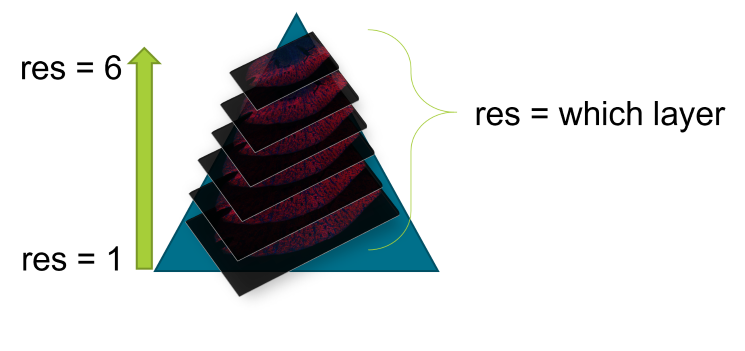
Pyramidal TIFF
The res variable says which resolution of the image to
extract. 1 = largest image, or the bottom of the OME-TIFF “pyramid”.
Higher res values indicate the smaller, lower resolution
versions of the image. Each OME-TIFF has a different number of layers,
with most GeoMx experiment files having around 8. It is suggested to use
the smallest res value (highest resolution) your
environment can handle. This is a trial and error process.
Using too big of an image will cause a java memory error. If this
error occurs, increase your res value. Below is an example
of the error you will receive if the resolution is too high for your own
system.
Error in .jcall("RBioFormats", "Ljava/lang/Object;", "readPixels", i,  :
  java.lang.NegativeArraySizeException: -2147483648
The resolution size will affect speed and image resolution through
the rest of the analysis. To check the smallest resolution size
available, for the fastest speeds, use checkValidRes(). For
the rest of this tutorial we will be using res = 4 for
vignette size restrictions; res 4-6 is generally
recommended.
Note: If res =4 is giving you an error, try restarting R
and/or increasing the res value (remember higher
res parameter = higher slice on OME-TIFF pyramid = smaller
and lower resolution image).
#lowest resolution = fastest speeds
checkValidRes(ometiff = tifFile)
res <- 4
muBrain <- addImageOmeTiff(overlay = muBrain, ometiff = tifFile, res = res)
muBrain
showImage(muBrain)
plotSpatialOverlay(overlay = muBrain, colorBy = "segment", corner = "topcenter",
                   scaleBarWidth = 0.5, textDistance = 130, scaleBarColor = "cyan")
Visualization Marker Legends
There are two ways to add a legend to the graph showing the immunofluorescence visualization markers used.
The first is an easy way for data exploration: adding a legend to the
ggplot object directly by setting flourLegend = TRUE.
plotSpatialOverlay(overlay = muBrain, colorBy = "segment", corner = "topcenter",
                   scaleBarWidth = 0.5, textDistance = 130, scaleBarColor = "cyan",
                   fluorLegend = TRUE)
The second requires more user manipulation, but creates a more
publication-ready figure. The flourLegend function creates
a separate plot that can be added to the graph. The legend shape can be
changed with nrow and the background can be changed using
boxColor and alpha.
See ?draw_plot for more instructions on how to
manipulate the legend position and scale.
library(cowplot)
gp <- plotSpatialOverlay(overlay = muBrain, colorBy = "segment",
                         corner = "bottomright")
legend <- fluorLegend(muBrain, nrow = 2, textSize = 4,
                      boxColor = "grey85", alpha = 0.3)
cowplot::ggdraw() +
    cowplot::draw_plot(gp) +
    cowplot::draw_plot(legend, scale = 0.105, x = 0.1, y = -0.25)
Image Manipulation
Flipping Axes
Images and overlays can be flipped across either axis to reorient the
image. To flip both axes, use flipY(flipX(overlay)). These
functions update the coordinates and image rather than just affecting
the figure. You cannot run these commands until the image is associated
with the spatial overlay object. If you want to reverse axes on a plot
that features only ROIs, and not the underlying image, you can run
plotSpatialOverlay() with the overlay object
flipped at will and the parameter image=FALSE.
In this example, the original image is reversed from the traditional view of the mouse brain, so we shall flip the y-axis.
muBrain <- flipY(muBrain)
plotSpatialOverlay(overlay = muBrain, colorBy = "segment", scaleBar = FALSE)
plotSpatialOverlay(overlay = flipX(muBrain), colorBy = "segment", scaleBar = FALSE)
Cropping
Images can be cropped in two ways. The amount of area added to the
cropped area in both methods can be defined by buffer. This
adds a percentage of the final image size to each edge.
-
cropTissue()automatically detects where the tissue is and removes the surrounding blank area.
muBrain <- cropTissue(overlay = muBrain, buffer = 0.05)
plotSpatialOverlay(overlay = muBrain, colorBy = "ROILabel", legend = FALSE, scaleBar = FALSE)+
viridis::scale_fill_viridis(option = "C")-
cropSamples()automatically crops the image around the ROIs given. Other ROIs in the cropped image can be kept in or ignored. Below we will crop to only ROIs that are unsegmented, hiding ROIs profiles that are segmented. SettingsampsOnly = TRUEhides the segmented ROIs within the plotted region.
samps <- muBrainAnnots$Sample_ID[muBrainAnnots$segment == "Full ROI" &
                                     muBrainAnnots$slide.name == slideName(muBrain)]

muBrainCrop <- cropSamples(overlay = muBrain, sampleIDs = samps, sampsOnly = TRUE)
plotSpatialOverlay(overlay = muBrainCrop, colorBy = "Calm1", scaleBar = TRUE,
                   corner = "bottomleft", textDistance = 5)+
    ggplot2::scale_fill_gradient2(low = "grey", high = "red",
                                  mid = "yellow", midpoint = 2500)

muBrainCrop <- cropSamples(overlay = muBrain, sampleIDs = samps, sampsOnly = FALSE)
plotSpatialOverlay(overlay = muBrainCrop, colorBy = "segment", scaleBar = TRUE,
                   corner = "bottomleft", textDistance = 5)
Image Coloring
Image colors and contrast settings are typically determined by user
on the GeoMx DSP instrument before exporting the OME-TIFF. However, the
SpatialOmicsOverlay package allows users to affect the
coloring during analysis.
This recoloring must be done on the 4-channel image before converting
to RGB. The color code and min/max intensities determine the coloring of
the RGB image. To view the current color definition use the
fluor function.
The color can be a hex color or a valid R color name. The dye can
either come from the Dye or DisplayName
columns from fluor(overlay). To change a color, use the
changeImageColoring function.
chan4 <- add4ChannelImage(overlay = muBrain)
fluor(chan4)
chan4 <- changeImageColoring(overlay = chan4, color = "#32a8a4", dye = "FITC")
chan4 <- changeImageColoring(overlay = chan4, color = "magenta", dye = "Alexa 647")
chan4 <- changeColoringIntensity(overlay = chan4, minInten = 500,
                                 maxInten = 10000, dye = "Cy5")
fluor(chan4)
# change 4 channel TIFF to RGB
chan4 <- recolor(chan4)
showImage(chan4)
Future Directions
In future releases of SpatialOmicsOverlay, we will
be:
- Ensuring capability with NanoString’s CosMx Spatial Molecular Imager outputs.
- Adding ability to add graphing features on top of the image.
- Adding image analysis capabilities.
- Adding extraction of image data to use in ML/AI applications.
For your reference:
NanoString Technologies, Inc.↩︎