
library(ggplot2)
library(ggrepel)
library(data.table)
library(HieraType)1 Abstract
This post showcases a hierarchical cell typing method (HieraType) optimized for detection and sub-clustering of immune cells. HieraType:
- Is organized around canonical marker genes, but harnesses cells’ complete expression profiles.
- Can be adapted to any arbitrary cell type hierarchy.
Code for the method and utility functions used in this post can be found in the R package HieraType. The package contains carefully designed pipelines for:
- Subclassifying T-cells into 12 categories
- Classifying a whole dataset into broad categories (epithelial, fibroblast, immune, endothelial), then subclassifying immune cells into 9 categories
- Classifying native brain cells
It is also possible to assemble pipelines for custom applications, e.g. focused on a specific tissue type.
In this post, we use a 6K-plex colon-cancer dataset to demonstrate two common use cases for the method:
- Subtyping T cells
- Broad immune cell typing.
2 Quick links to the code
For those in a hurry to ‘just see the code’, they can jump ahead to the “Just The Code” sections for Example 1, or Example 2.
3 Introduction
Often (particularly with immune cells), we may want our cell type calls to be guided by specific sets of marker genes.
In some spatially-resolved transcriptomics (SRT) datasets, directly using marker gene expression for determining cell type may be a challenge due to data sparsity, background, or segmentation ambiguity. These challenges together can make marker genes noisy individual data points.
However, marker genes remain a strong organizing principle for differentiating cell types. To overcome the intrinsic noise of single marker genes, the cell typing method we describe here captures information from both (a) similar cells and (b) biologically relevant genes, in order to construct metagenes that more stably estimate true marker expression. These marker metagene scores are then used for probabilistic cell type assignment. The method takes as input predefined ‘marker lists’ for each cell type, which make it easy to enforce prior biological assumptions about the marker genes and expression profiles we expect to see in our cell types. By not requiring any training data or an explicit reference profile, we expect the method to be robust to platform or batch effects that may otherwise challenge cell type labeling from pre-trained models or external reference data.
The basic framework for the method can be described in a few basic steps (we’ll describe each of these steps in more detail throughout our examples.)
- First, for each cell type, we define a set of genes we expect may be ‘marker genes’ or highly expressed based on prior data or biology (either the literature, a reference dataset, or some combination of both).
- Next, we construct metagene scores from our data for each cell type based on the genes specified in (1).
- Finally, we model the metagene scores, where the model estimates a posterior probability that each cell belongs to any of the possible cell types.
We’ll use an internally generated colon cancer dataset profiled with the CosMx Human 6K Discovery Panel comprised of about 112k cells, and work through two common cell typing scenarios in which we envision this methodology can be useful:
- Subclustering an existing set of cell types:
- In this first case, we’ll assume we’ve already done some basic clustering, but don’t quite have the level of cell type granularity we’d like. We’ll take a ‘T cell’ cluster and sub-classify those cells into CD8-T and CD4-T, followed by more granular T cell subcategories.
- Top down hierarchical cell typing with focus on immune cells:
- Here we’ll start from scratch; first assigning cells into major categories and identifying immune cells, then classifying those immune cells into various sub classifications of myeloid and lymphocyte cell types.
4 Initial look at our dataset
Let’s start by taking an initial look at our data, then walk through some cell typing scenarios. First, we can load in our data and take a look at some unsupervised leiden clustering we’ve already performed.
## Note, using a v3-style Seurat Object below, i.e., `sem[["RNA"]]@counts`
## For v5-style, the syntax would be like `sem[["RNA"]]$counts`
options(Seurat.object.assay.version = "v3")

sem <- readRDS("colon_seurat.rds")
normed <- HieraType::totalcount_norm(Matrix::t(sem[["RNA"]]@counts))
sem <- Seurat::SetAssayData(sem, layer = "data", new.data = Matrix::t(normed))
Spatial plot of initial clusters
Here’s a spatial plot of our leiden clusters. At first glance, we see that some of these unsupervised clusters (i.e., 3, 0, 1, 2, and 7 for example) have distinct spatial patterns; it definitely looks like some meaningful biological structure in these tissue were captured by unsupervised clustering.
Code
sem@meta.data$portion <- "part_a"
sem@meta.data$portion[sem@meta.data$fov %in% 60:73] <- "part_b"
xyplist <-
lapply(split(data.table(sem@meta.data), by = "portion"), function(xx){
  HieraType::xyplot("clusters_unsup", metadata = xx,ptsize = 0.1) + coord_fixed()
})
xypl <-
cowplot::plot_grid(plotlist=xyplist, nrow=1) +
theme(plot.background = element_rect(fill = 'white',color='white')) +
  cowplot::panel_border(remove=TRUE)
print(xypl)
Heatmap of initial clusters
We can make a marker gene heatmap to identify some of the top marker genes for each cluster and see if we recognize any of the celltypes represented by the unsupervised clusters. Here we can use a couple of convenience functions provided in the R package HieraType.
Code
## calculate fold change, average expression, and other summary metrics
## for each gene and each cluster compared to other clusters
## This is the data underlying the marker heatmap.
fctbl_unsup <-
HieraType::clusterwise_foldchange_metrics(normed  = sem[["RNA"]]@data
                                          ,metadata = sem@meta.data
                                          ,cluster_column = "clusters_unsup"
                                          )

## make a marker heatmap
hm_unsup <- HieraType::marker_heatmap(fctbl_unsup
                           ,extras = c("CD3D", "CD4", "FOXP3"
                                       , "CD8B", "CD8A")
                           )
print(hm_unsup)
Let’s suppose for sake of demonstration that I recognize (and am comfortable enough) to label these clusters with cell type names based on the marker genes shown in the heatmap.
However, there are one or a few of my immune clusters I’ve identified where I desire more granularity. In this case, I’m particularly interested in my T cells; in the bottom-left hand corner of the heatmap plot above, I see that ‘cluster 6’ is capturing T-cells, showing enrichment in some key marker genes like CD3 (CD3D, CD3E) as well as other markers like CD2, IL7R, and ITK.
I’d like to split these cells further into at least a few meaningful T-cell subtypes, at minimum: “CD8+”, “CD4+”, and “Treg”.
5 Example case 1: Subclustering T cells
5.1 ‘Just The Code’
Here’s the code for classifying leiden cluster ‘6’ into cd8t and cd4t cell types , followed by more granular T cell subtyping. We use the R package HieraType with a prespecified tcell_pipeline, and corresponding lists of marker genes included as package datasets. A pipeline specifies the hierarchical order we want to do our cell typing, and which cell types go in each level of the hierarchy. Each cell type has a list of associated marker genes.
data("pipeline_tcell")str(pipeline_tcell, max.level = 2)List of 3
$ markerslists :List of 3
..$ tmajor :List of 2
.. ..- attr(*, "class")= chr [1:2] "list" "markerslist"
..$ t4minor:List of 7
.. ..- attr(*, "class")= chr [1:2] "list" "markerslist"
..$ t8minor:List of 5
.. ..- attr(*, "class")= chr [1:2] "list" "markerslist"
$ priors :List of 2
..$ t4minor: chr "tmajor"
..$ t8minor: chr "tmajor"
$ priors_category:List of 2
..$ t4minor: chr "cd4t"
..$ t8minor: chr "cd8t"
- attr(*, "class")= chr [1:2] "list" "pipeline"names(pipeline_tcell$markerslists$tmajor)[1] "cd8t" "cd4t"names(pipeline_tcell$markerslists$t4minor)[1] "cd4_naive" "cd4_tem" "cd4_tcm" "cd4_th1" "cd4_th2" "cd4_th17"
[7] "cd4_treg" names(pipeline_tcell$markerslists$t8minor)[1] "cd8_naive" "cd8_tem" "cd8_tcm" "cd8_cytotoxic"
[5] "cd8_exhausted"### these are cells I want to subcluster
tcell_ids <- sem@meta.data[sem@meta.data$clusters_unsup==6,"cell_ID"]
### Run a 'tcell'-typing pipeline, which
### first classifies into T8/T4 categories (using the `tmajor` markerslist),
### then runs subclassification for T4 and T8 using the t4minor and t8minor markerslists.
tcell_typing <-
run_pipeline(pipeline = pipeline_tcell
,counts_matrix = Matrix::t(sem[["RNA"]]@counts[,tcell_ids])
,adjacency_matrix = as(sem@graphs$umapgrph
,"CsparseMatrix")[tcell_ids,tcell_ids]
,celltype_call_threshold = 0.5
)The data table post_probs in our tcell_typing object holds the high-level cell typing results; the celltype_thresh column shows the most granular cell type call where posterior probability is \(> 0.5\) (our celltype_call_threshold). We can see the posterior probablity for the celltype_thresh category in best_score_thresh.
The best granular cell type call (regardless of score) is given by the celltype_granular column, with best_score_granular indicating the corresponding posterior probability.
str(tcell_typing, max.level = 2)List of 3
$ post_probs :List of 1
..$ tmajor:Classes 'data.table' and 'data.frame': 7356 obs. of 5 variables:
.. ..- attr(*, ".internal.selfref")=<externalptr>
.. ..- attr(*, "sorted")= chr "cell_ID"
$ models :List of 3
..$ tmajor :List of 3
..$ t4minor:List of 3
..$ t8minor:List of 3
$ metagene_scores:List of 3
..$ tmajor :List of 2
..$ t4minor:List of 7
..$ t8minor:List of 5tcell_typing$post_probs$tmajor[1:10][]Key: <cell_ID>
cell_ID celltype_thresh celltype_granular best_score_granular
<char> <char> <char> <num>
1: c_1_12_1014 cd8t cd8_exhausted 0.4691963
2: c_1_12_1066 cd4t cd4_th1 0.3352265
3: c_1_12_1091 cd4_th2 cd4_th2 0.9683195
4: c_1_12_1175 cd8_cytotoxic cd8_cytotoxic 0.8777777
5: c_1_12_1270 cd8_tem cd8_tem 0.5882417
6: c_1_12_1286 cd4_treg cd4_treg 0.9909980
7: c_1_12_1325 cd4t cd4_tcm 0.4647576
8: c_1_12_1346 cd4_treg cd4_treg 0.8298557
9: c_1_12_1349 cd8t cd8_tem 0.3939835
10: c_1_12_1394 cd8_cytotoxic cd8_cytotoxic 0.9587283
best_score_thresh
<num>
1: 0.9999999
2: 0.6751557
3: 0.9683195
4: 0.8777777
5: 0.5882417
6: 0.9909980
7: 0.9984388
8: 0.8298557
9: 0.9999814
10: 0.9587283Now lets take a closer look at the details and describe the methodology for each step.
5.2 Detailed walkthrough
5.2.1 Part 1: Specifying genes associated with my cell types based on prior biology
We’ll describe the first level of cell type classification from our example above to illustrate the method, where we suppose we want to classify cd4t vs. cd8t. Creating a marker list, by specifying genes I expect might be associated with my cell types is the first step of this algorithm. For each of my cell types, cd4t and cd8t, I specify
- a set of primary defining markers or “index genes” (these are genes that should be fairly exclusive to the cell type if possible)
- a set of other marker genes which I expect could be expressed as “predictors”
In this case, we’ll use [CD4], and [CD8A, CD8B], as “index genes” for cd4t and cd8t respectively. The other genes we’ll specify as predictors are based on the literature. For example, FOXP3 is often associated with cd4t ‘Treg’ cells, so we include it as a predictor here for cd4t. In general, it’s okay to include a gene as a “predictor” even if we only expect to see it in a subset of cells (like FOXP3 in this example, which we expect to be present in a ‘Treg’ subtype, but not all cd4t cells).
It’s okay to include markers in multiple cell types if that fits our mental model. For example, CD3D, CD3E, and CD3G are general T cell markers, and so are included as predictors for both subtypes, as are other genes like IL7R, CD27, SELL which could be seen in either cd4t or cd8t cells. When manually creating a marker list, consider “more predictors is better” as a general rule of thumb; a larger number of predictor genes can help build more accurate metagene models for celltype index markers.
We can create our marker list manually like this:
markerslist_tcellmajor <-
HieraType::make_markerslist(
  index_marker = list(
    "cd8t" = c("CD8B", "CD8A")
    ,"cd4t" = c("CD4")
  )
  ,predictors = list(
    "cd8t" =  c("CD3D", "CD3E", "CD3G", "CD8A", "CD8B", "IL7R", "CD27", "SELL", "CCR7", "TCF7", "LEF1",
                    "FOXP1", "BACH2", "KLF2", "CD28", "ICOS", "STAT3", "STAT5", "RUNX3", "BATF", "EOMES",
                    "TBX21", "PRDM1", "PDCD1", "LAG3", "TIGIT", "HAVCR2", "GZMK", "GZMA", "GZMB", "PRF1",
                    "GNLY", "KLRG1", "KLRD1", "IFNG", "CCL5", "CX3CR1", "NKG7", "FAS", "FASLG", "IL2", "CD244",
                    "CXCR3", "KLRB1", "TOX", "NR4A2", "BCL6", "CXCL13")
    ,"cd4t" = c("CD3D", "CD3E", "CD3G", "CD4", "IL7R", "CD27", "SELL", "CCR7", "TCF7", "LEF1", "FOXP1",
                     "BACH2", "KLF2", "CD28", "ICOS", "CD40LG", "STAT3", "STAT5", "RUNX1", "RUNX3", "BATF",
                     "GATA3", "TBX21", "RORC", "FOXP3", "IL2RA", "CTLA4", "PDCD1", "LAG3", "TIGIT", "HAVCR2",
                     "IL2", "IFNG", "IL4", "IL5", "IL13", "IL17A", "IL17F", "IL10", "CCL5", "CXCR3", "CCR6",
                     "CXCR5", "PRDM1", "BCL6", "EOMES", "CXCL13", "TOX")
  )
)
The object created looks like this below
str(markerslist_tcellmajor)List of 2
$ cd8t:List of 3
..$ index_marker : chr [1:2] "CD8B" "CD8A"
..$ predictors : chr [1:48] "CD3D" "CD3E" "CD3G" "CD8A" ...
..$ use_offclass_markers_as_negative_predictors: logi TRUE
$ cd4t:List of 3
..$ index_marker : chr "CD4"
..$ predictors : chr [1:48] "CD3D" "CD3E" "CD3G" "CD4" ...
..$ use_offclass_markers_as_negative_predictors: logi TRUE
- attr(*, "class")= chr [1:2] "list" "markerslist"In practice, we can save and reuse our marker lists for different cell types. While it should be easy to create/modify a custom list from the literature, this particular list is included as a package dataset markerslist_tcellmajor to facilitate ease of use.
data("markerslist_tcellmajor")str(markerslist_tcellmajor)List of 2
$ cd8t:List of 3
..$ index_marker : chr [1:2] "CD8B" "CD8A"
..$ predictors : chr [1:48] "CD3D" "CD3E" "CD3G" "CD8A" ...
..$ use_offclass_markers_as_negative_predictors: logi TRUE
$ cd4t:List of 3
..$ index_marker : chr "CD4"
..$ predictors : chr [1:48] "CD3D" "CD3E" "CD3G" "CD4" ...
..$ use_offclass_markers_as_negative_predictors: logi TRUE
- attr(*, "class")= chr [1:2] "list" "markerslist"5.2.2 Part 2: Estimating a metagene score for each cell type
Because single count values marker genes can be noisy, we seek to derive variables that more stably estimate marker expression. To do so, we’ll exploit biologically relevant genes (e.g. CD8A expression is predictive of CD8B expression), and cells with similar expression patterns. To do so, we fit a model for each cell type, using the primary index marker as the response variable and covariates derived from the predictor genes. The predicted values of the primary index marker for this model make a continuous “metagene score” that will later be used for probabilistic cell type assignment. You can think of each metagene score as estimating the canonical marker gene’s expression for a single cell type; e.g. we will produce a FOXP3-estimating metagene to capture Treg’s, a CD68-estimating metagene to capture macrophages, etc…
We fit our models for each cell type class using the fit_metagene_scores function. This function uses ‘smoothing’ (averaging over a set of similar cells), as well as our prior biology / assumptions about which markers are associated with each celltype to predict the pearson residuals of the index gene.
The default regression model setup looks like this: \[Y = WY\eta + WX\beta + X\gamma + \epsilon \] where
- \(Y:=\) pearson residuals of the index marker (our response variable)
- \(X:=\) (totalcount-normalized) matrix of predictor genes
- \(W:=\) a cells \(\times\) cells neighborhood matrix, denoting cells with similar expression profiles.
- \(\eta\), \(\beta\), and \(\gamma\) are the regression coefficients associated with the ‘neighbor-averaged’ index gene, ‘neighbor-averaged’ predictor genes, and predictor genes within the cell respectively.
One way to think about this model specification could be as an implementation of a ‘smoothing model’, which leverages information across multiple dimensions:
- the index gene’s mean expression in similar cells (\(WY\)) (roughly, neighbors in UMAP space)
- expression of other expected marker genes (\(X\)) (our predictor genes defined from biological knowledge)
- expression of other expected marker genes in similar cells (\(WX\))
We use a non-negative least squares (Slawski and Hein 2013) (NNLS) regression to estimate our models. The NNLS model enforces that all of the covariates based on predictor genes we specified must have positive regression coefficients (in practice we’ll observe that a number of regression coefficients may shrink to zero).
By specifying use_offclass_markers_as_negative_predictors = TRUE in the section above, we further assume that predictors for other celltypes that we haven’t listed can be used as negative predictors of our index gene. For example, genes like like “GZMA” and “GZMB”, which are markers associated with cd8t, will be assumed to be negative predictors of the other classes (cd4t) where they are not listed. This argument should in general be set to TRUE, as it’s useful to specify which genes we don’t expect to see in a celltype. If your markers list has extensive genes expected to be enriched in multiple cell types, and those genes are for some reason omitted from many of the other cell types, then a user might consider specifying this argument as FALSE; e.g. if many genes like CD3E are specified in markers lists for some T cell subtypes but not all (despite being ubiquitously expressed).
Estimating this model from the dataset at hand rather than using a reference model could make this framework more robust to platform effects or batch effects compared to pre-trained models or reference profiles which used different technology or data with slightly different biology.
Genes not included in the marker gene lists will not be considered in assigning cell types. Because the model is only using genes we’ve specified in our ‘markers list’, we have complete control over which genes influence the metadata scores, reducing the chance that noisy or irrelevant genes can have an impact on our cell type classifications. Furthermore, by estimating the metagenes directly from the dataset at hand, we are not reliant on reference datasets or pre-trained models influenced by different technology (example: scRNA-seq) or underlying biology (example: different tissue type or disease status, etc).
Here I call the fit_metagene_scores function to estimate these models for cells corresponding to the unsupervised cluster I’ve identified to be T cells.
For the cells \(\times\) cells adjacency_matrix, I’ve used the nearest neighbor matrix in my Seurat object. This is the same graph that was used to generate my UMAP and my unsupervised leiden clusters. After fitting our regression models for each cell type, we’ll use the predicted scores as ‘metagenes’ that can be clustered in the next step.
tcell_ids <- sem@meta.data[sem@meta.data$clusters_unsup==6,"cell_ID"]
metagenes_t <-
  fit_metagene_scores(
    markerslist = markerslist_tcellmajor
    ,counts_matrix = Matrix::t(sem[["RNA"]]@counts[,tcell_ids])
    ,adjacency_matrix = as(sem@graphs$umapgrph
                           ,"CsparseMatrix")[tcell_ids,tcell_ids]
  )
The metagenes_t object we’ve created has an element for each celltype, including the regression coefficients (bhat), and predicted values we’ll use for clustering (yhat) for each index marker gene for cell type.
str(metagenes_t,max.level = 2)List of 2
$ cd8t:List of 7
..$ CD8B :List of 5
..$ CD8A :List of 5
..$ yhat : Named num [1:7356] 0.593 1.32 2.959 1.375 2.478 ...
.. ..- attr(*, "names")= chr [1:7356] "c_1_12_1066" "c_1_12_1175" "c_1_12_1270" "c_1_12_1349" ...
..$ y : Named num [1:7356] -0.208 -0.178 2.047 -0.207 -0.242 ...
.. ..- attr(*, "names")= chr [1:7356] "c_1_12_1066" "c_1_12_1175" "c_1_12_1270" "c_1_12_1349" ...
..$ ypost : Named num [1:7356] -0.1796 -0.0223 1.5179 -0.0269 0.1805 ...
.. ..- attr(*, "names")= chr [1:7356] "c_1_12_1066" "c_1_12_1175" "c_1_12_1270" "c_1_12_1349" ...
..$ bhat : num [1:125, 1:2] 0.1904 0.1342 0.1113 0.1057 0.0912 ...
.. ..- attr(*, "dimnames")=List of 2
..$ nnpcfit:List of 7
.. ..- attr(*, "class")= chr [1:2] "nsprcomp" "prcomp"
$ cd4t:List of 6
..$ CD4 :List of 5
..$ yhat : Named num [1:7356] 0.29 -1.426 -0.968 -0.692 -1.945 ...
.. ..- attr(*, "names")= chr [1:7356] "c_1_12_1066" "c_1_12_1175" "c_1_12_1270" "c_1_12_1349" ...
..$ y : Named num [1:7356] -0.271 -0.235 -0.418 -0.27 -0.312 ...
.. ..- attr(*, "names")= chr [1:7356] "c_1_12_1066" "c_1_12_1175" "c_1_12_1270" "c_1_12_1349" ...
..$ ypost : Named num [1:7356] -0.294 -0.366 -0.469 -0.321 -0.507 ...
.. ..- attr(*, "names")= chr [1:7356] "c_1_12_1066" "c_1_12_1175" "c_1_12_1270" "c_1_12_1349" ...
..$ bhat : num [1:125, 1] 0.3763 0.2525 0.1551 0.1283 0.0749 ...
.. ..- attr(*, "dimnames")=List of 2
..$ nnpcfit:List of 7
.. ..- attr(*, "class")= chr [1:2] "nsprcomp" "prcomp"For cell types using multiple ‘index marker genes’, like cd8t here (using CD8A and CD8B), metagene scores are combined together using non-negative sparse pca (implemented in the nsprcomp R package) (Sigg and Buhmann 2008). This allows for summarizing an overall cell type metagene score, using a constrained non-negative combination of individual index-gene scores that explains maximal variation across individual index gene scores. Below, we see the PCA rotation representing the individual weights given to CD8A and CD8B metagene scores.
metagenes_t$cd8t$nnpcfitStandard deviations (1, .., p=1):
[1] 1.020128
Rotation (n x k) = (2 x 1):
PC1
CD8B 0.6578375
CD8A 0.7531599We can get a better understanding of the metagene model outputs by looking at a few diagnostics plots. In the below, we plot the regression coefficients for each model, ordering them on the x-axis by their ranking. For each cell type, the positive \(\hat{\beta}\) correspond to genes we specified as predictors, and negative \(\hat{\beta}\) were predictors for either of the other two cell types.
A lot of the covariates which have the largest magnitudes have “lag.” in their name indicating they correspond to a smoothed (or neighbor-averaged) covariate for that gene.
We also see that many genes end up with weights of 0. These genes failed to be predictive in the direction our biological priors expected.
For cd4t, we see that smoothed CD4 (indicated by ‘lag.y.CD4’ in the plot) is the strongest predictor of observed ‘CD4’. For cd8t, ‘lag.y.CD8A’ and ‘lag.y.CD8B’ (indicating smoothed CD8A and CD8B) are also among the strongest predictors, but not first in rank.
Code
coefplots <- metagene_coefficients_plot(metagenes_t)
coefplots <- lapply(coefplots, function(x){x +   theme(text=element_text(face='bold',size=18))
  }) ## just make the text bigger and bold
cowplot::plot_grid(plotlist = coefplots, nrow = 1)
A pairsplot can show us how well the metagene scores we’ve created are distinct from each other. Ideally, if our cell type classes are mutually exclusive, we’d want to not see too many cells which are ‘positive’ for multiple cell types at the same time.
Here, we see that cd4t and cd8t metagene scores are negatively correlated with each other, which is good to see.
Code
metagene_pairsplot(metagenes_t, var= "yhat")
5.2.3 Part 3: Assigning cell types based on metagene scores
Now we use the metagene scores to classify cell types. To do so, we estimate the multivariate distribution of metagene scores that characterize each cell type. This allows us to compute the likelihoods for a cell belonging to any of these types, and infer a posterior probability of T-cell subtype for each cell. The cluster_metagenes function we run below estimates a mixture of overfitted multivariate gaussian mixture models (Aragam et al. 2020) to estimate the distribution of metagene scores.
model_t <-
HieraType::cluster_metagenes(metagenes = metagenes_t)
At a high level, the cluster_metagenes() function first identifies all cells with positive metagene scores for a particular cell type. We might loosely interpret these cells as ‘anchor cells’. The data may look like this for example, where here I have subset my original data to cells which have positive scores for my celltype cd8t.
yh <- make_scores_matrix(metagenes = metagenes_t, "yhat")
yh[yh[,"cd8t"] > 0,][1:10,]
Then, a mixture model is fit to these (2-dimensional) scores, by default using 6 components. The estimates corresponding to the individual mixture models for each cell type are found in the models list, with the means (mu_hat), covariance matrices (sigma_hat), and prior probability (pihat) corresponding to each mixture component.
str(model_t$models, max.level = 2)List of 2
$ cd8t:List of 6
..$ post_probs :Classes 'data.table' and 'data.frame': 2528 obs. of 9 variables:
.. ..- attr(*, ".internal.selfref")=<externalptr>
..$ pihat : Named num [1:6] 0.2785 0.103 0.0437 0.3024 0.0747 ...
.. ..- attr(*, "names")= chr [1:6] "k1" "k2" "k3" "k4" ...
..$ llmat : num [1:2528, 1:6] -2.97 -2.87 -2.95 -3.42 -2.43 ...
.. ..- attr(*, "dimnames")=List of 2
..$ mu_hat : num [1:6, 1:2] 2.136 0.136 2.966 1.196 0.645 ...
.. ..- attr(*, "dimnames")=List of 2
..$ sigma_hat :List of 6
..$ loglik_iters: num [1:262] -4920 -4891 -4883 -4879 -4876 ...
$ cd4t:List of 6
..$ post_probs :Classes 'data.table' and 'data.frame': 2623 obs. of 9 variables:
.. ..- attr(*, ".internal.selfref")=<externalptr>
..$ pihat : Named num [1:6] 0.1544 0.1398 0.2798 0.0414 0.0677 ...
.. ..- attr(*, "names")= chr [1:6] "k1" "k2" "k3" "k4" ...
..$ llmat : num [1:2623, 1:6] -2.03 -56.28 -126.91 -3.61 -5.12 ...
.. ..- attr(*, "dimnames")=List of 2
..$ mu_hat : num [1:6, 1:2] -1.074 -0.779 -1.13 -1.796 -1.429 ...
.. ..- attr(*, "dimnames")=List of 2
..$ sigma_hat :List of 6
..$ loglik_iters: num [1:173] -5230 -5189 -5167 -5155 -5147 ...Typically we shouldn’t need to interact with this part of the output. After the mixture models for each cell type are fitted, we can score all cells, and get an overall posterior probability that a cell belongs to any of the two major classes using Bayes rule.
Let \(y_c\) be the cell type category for cell \(c\), \(scores_c\) the corresponding metagene scores, and \(t\) denoting a possible cell ‘type’ or category (for \(t = 1,...,T\)).
We compute the overall posterior probability that \(y_c\) is a particular type \(t\), as
\[P(y_c = t | scores_c) = \frac{P(scores_c | y_c = t)P(y_c = t)}{\sum_{l=1}^T P(scores_c | y_c = l)P(y_c = l)}\]
Using the individual mixture models for a particular cell type with \(K\) mixture components, we have \[P(scores_c | y_c = t) = \sum_{j=1}^K P(scores_c | k=j, y_c = t) P(k=j | y_c = t)\]
The prior probability for a particular cell type class \(t\) can be estimated by counting the number of cells used to estimate the mixture model in each cell type, and computing a proportion amongst all possible cell type classes, i.e., \[P(y_c = t) = \frac{\sum_{c=1}^C I(scores_{c,t} > 0)}{\sum_{l=1}^T \sum_{c=1}^C I(scores_{c,l} > 0)}\] These probabilities are in the post_probs data.table object of the model. The “best class” column gives each cell’s best-fitting cell type.
model_t$post_probs[1:10][] cell_ID best_class best_score cd8t cd4t
<char> <char> <num> <num> <num>
1: c_1_12_1066 cd4t 0.6751557 0.324844253 6.751557e-01
2: c_1_12_1175 cd8t 0.9999986 0.999998637 1.363123e-06
3: c_1_12_1270 cd8t 0.9999989 0.999998939 1.060938e-06
4: c_1_12_1349 cd8t 0.9999814 0.999981384 1.861648e-05
5: c_1_12_1394 cd8t 1.0000000 0.999999986 1.438074e-08
6: c_1_12_172 cd4t 0.9979380 0.002061995 9.979380e-01
7: c_1_12_228 cd4t 0.9955272 0.004472831 9.955272e-01
8: c_1_12_246 cd4t 0.9933210 0.006679029 9.933210e-01
9: c_1_12_285 cd4t 0.9986854 0.001314640 9.986854e-01
10: c_1_12_511 cd4t 0.9911673 0.008832705 9.911673e-015.2.4 Granular hierarchical subtyping and using a pipeline
These posterior-probability scores can be passed directly to subtyping models for cd4t and cd8t, via the prior_level_weights arguments. For example, if I wanted to go ahead and cluster the cd4t cells into subtypes, I could follow the same process, passing in the prior probability of the cell being cd4t as a weight.
In the example below, the probability of cd4t is used as a weight in the NNLS regression fitting (akin to weighted least squares) when constructing metagene scores. Cells with high probability of cd4t are emphasized, while cells with lower probability of cd4t have less influence on the regression coefficients used to generate metagene scores.
In the clustering stage, probability of cd4t is again used as a weight (or prior probability), that factors into the expectation step of the EM algorithm. Letting s(t) denote the subtype of cd4t, then we have the below, where \(P(y_c = t)\) would be the probability of cd4t from the previous stage of modeling.
The final returned probability for each cd4t subtype is a joint probability of both being the subtype \(s(t)\) and the major celltype \(t\).
\[P(y_c = s(t) \cap y_c = t | scores_c) = P(y_c = s(t) | scores_c, y_c = t)P(y_c = t)\]
Below is an example of this syntax using the cd4t subtypes in the package dataset “markerslist_cd4tminor”.
str(HieraType::markerslist_cd4tminor, max.level=2)List of 7
$ cd4_naive:List of 3
..$ index_marker : chr [1:4] "TCF7" "LEF1" "SELL" "CCR7"
..$ predictors : chr [1:30] "CD3D" "CD3E" "CD3G" "CD4" ...
..$ use_offclass_markers_as_negative_predictors: logi TRUE
$ cd4_tem :List of 3
..$ index_marker : chr [1:4] "CD44" "CCR6" "CXCR3" "IL7R"
..$ predictors : chr [1:35] "CD3D" "CD3E" "CD3G" "CD4" ...
..$ use_offclass_markers_as_negative_predictors: logi TRUE
$ cd4_tcm :List of 3
..$ index_marker : chr [1:3] "CCR7" "IL7R" "SELL"
..$ predictors : chr [1:27] "CD3D" "CD3E" "CD3G" "CD4" ...
..$ use_offclass_markers_as_negative_predictors: logi TRUE
$ cd4_th1 :List of 3
..$ index_marker : chr [1:4] "TBX21" "IFNG" "CXCR3" "STAT4"
..$ predictors : chr [1:30] "CD3D" "CD3E" "CD3G" "CD4" ...
..$ use_offclass_markers_as_negative_predictors: logi TRUE
$ cd4_th2 :List of 3
..$ index_marker : chr [1:5] "GATA3" "IL4" "IL5" "IL13" ...
..$ predictors : chr [1:30] "CD3D" "CD3E" "CD3G" "CD4" ...
..$ use_offclass_markers_as_negative_predictors: logi TRUE
$ cd4_th17 :List of 3
..$ index_marker : chr [1:4] "RORC" "IL17A" "IL17F" "IL23R"
..$ predictors : chr [1:28] "CD3D" "CD3E" "CD3G" "CD4" ...
..$ use_offclass_markers_as_negative_predictors: logi TRUE
$ cd4_treg :List of 3
..$ index_marker : chr [1:4] "FOXP3" "IL2RA" "CTLA4" "TNFRSF18"
..$ predictors : chr [1:29] "CD3D" "CD3E" "CD3G" "CD4" ...
..$ use_offclass_markers_as_negative_predictors: logi TRUE
- attr(*, "class")= chr [1:2] "list" "markerslist"#### Classify cd4t subtypes
metagenes_t4 <-
HieraType::fit_metagene_scores(
markerslist = HieraType::markerslist_cd4tminor
,counts_matrix = Matrix::t(sem[["RNA"]]@counts[,tcell_ids])
,adjacency_matrix = as(sem@graphs$umapgrph
,"CsparseMatrix")[tcell_ids,tcell_ids]
,prior_level_weights = model_t$post_probs$cd4t ## prior probability of cd4t
)
model_t4 <-
HieraType::cluster_metagenes(metagenes = metagenes_t4, prior_prob_level = model_t$post_probs$cd4t)A convenient way to simplify this process with minimal code is to use a pipeline object. A custom hierarchical cell typing pipeline could be created like this below, where
markerslistsis a named list, with amarkerslistfor each stage of cell typing. “tmajor” will classifycd8tvs.cd4t, while “t8minor” and “t4minor” will subclassify those cell types respectively.priors, a list specifying ‘parent’ celltyping stage. Here ,t4minorandt8minorboth need to run after “tmajor”, as they will use the estimated probabilities of “cd4t” and “cd8t” as inputs.
“tmajor” runs first, and does not have prior probability inputs.priors_category, a list specifying ‘parent’ / major categories of each celltype. Here ,t4minoris a subset of"cd4t". “tmajor” runs first, and does not have a prior.
pipeline_tcell <-
  make_pipeline(markerslists = list("tmajor" = HieraType::markerslist_tcellmajor
                    ,"t4minor" = HieraType::markerslist_cd4tminor
                    ,"t8minor" = HieraType::markerslist_cd8tminor
                    )
                 ,priors = list("t4minor" = "tmajor"
                               ,"t8minor" = "tmajor")
                 ,priors_category = list("t4minor" = "cd4t"
                                         ,"t8minor" = "cd8t"
                                         )
)class(pipeline_tcell)[1] "list" "pipeline"This particular pipeline is also saved as a package dataset.
str(HieraType::pipeline_tcell, max.level=2)List of 3
$ markerslists :List of 3
..$ tmajor :List of 2
.. ..- attr(*, "class")= chr [1:2] "list" "markerslist"
..$ t4minor:List of 7
.. ..- attr(*, "class")= chr [1:2] "list" "markerslist"
..$ t8minor:List of 5
.. ..- attr(*, "class")= chr [1:2] "list" "markerslist"
$ priors :List of 2
..$ t4minor: chr "tmajor"
..$ t8minor: chr "tmajor"
$ priors_category:List of 2
..$ t4minor: chr "cd4t"
..$ t8minor: chr "cd8t"
- attr(*, "class")= chr [1:2] "list" "pipeline"The code to run the pipeline is shown below. Additional arguments to be passed to fit_metagene_scores or cluster_metagenes functions can be passed as additional arguments to run_pipeline() .
### Run a 'tcell'-typing pipeline, which
### first classifies into T8/T4 categories (using the `tmajor` markerslist),
### then runs subclassification for T4 and T8 using the t4minor and t8minor markerslists.
tcell_typing <-
run_pipeline(pipeline = pipeline_tcell
    ,counts_matrix = Matrix::t(sem[["RNA"]]@counts[,tcell_ids])
    ,adjacency_matrix = as(sem@graphs$umapgrph
                           ,"CsparseMatrix")[tcell_ids,tcell_ids]
    ,celltype_call_threshold = 0.5
    ,return_all_columns_postprobs = FALSE
    )
We could take a look at individual models and metagenes objects if needed within our tcell_typing result. Below, we show that the outputted objects are the same in the pipeline format, as if we had ran them individually like in the method demonstration.
all.equal(model_t, tcell_typing$models$tmajor)[1] TRUEall.equal(metagenes_t, tcell_typing$metagene_scores$tmajor)[1] TRUEBy default, two possible cell type classifications are returned in the overall post_probs data.table object from our pipeline. Below, celltype_granular shows the most granular classification for each cell, carrying the ‘best possible’ classification at each stage of the pipeline. For example, the first cell below was first identified as cd8t being the best category. The best subcategory of cd8t was cd8_exhausted, and the posterior probability score for cd8t_exhausted was ~0.47.
We set the the cutoff celltype_call_threshold=0.5 when we ran the pipeline, so that the celltype_thresh classification shows the most granular cell type with probability scores at least this threshold. The first cell below has cd8_exhausted score ~0.47 (less than 0.5), and so takes the higher level category of cd8t, which is above the threshold at ~0.99999.
tcell_typing$post_probs[["tmajor"]][1:10]Key: <cell_ID>
cell_ID celltype_thresh celltype_granular best_score_granular
<char> <char> <char> <num>
1: c_1_12_1014 cd8t cd8_exhausted 0.4691963
2: c_1_12_1066 cd4t cd4_th1 0.3352265
3: c_1_12_1091 cd4_th2 cd4_th2 0.9683195
4: c_1_12_1175 cd8_cytotoxic cd8_cytotoxic 0.8777777
5: c_1_12_1270 cd8_tem cd8_tem 0.5882417
6: c_1_12_1286 cd4_treg cd4_treg 0.9909980
7: c_1_12_1325 cd4t cd4_tcm 0.4647576
8: c_1_12_1346 cd4_treg cd4_treg 0.8298557
9: c_1_12_1349 cd8t cd8_tem 0.3939835
10: c_1_12_1394 cd8_cytotoxic cd8_cytotoxic 0.9587283
best_score_thresh
<num>
1: 0.9999999
2: 0.6751557
3: 0.9683195
4: 0.8777777
5: 0.5882417
6: 0.9909980
7: 0.9984388
8: 0.8298557
9: 0.9999814
10: 0.9587283We can remake this table with a different cutoff in mind as needed, depending on how conservative / aggressive we are comfortable being with the cell type call, using the combine_postprob_tables function.
As demonstration, we can look at the output if we were to raise our threshold from 0.5 to 0.8.
We can “return_all_columns” to show a more verbose result, with individual columns showing the joint probability scores for all possible cell type categories in each cell.
HieraType::combine_postprob_tables(pipeline = pipeline_tcell
                                   ,models = tcell_typing$models
                                   ,celltype_call_threshold = 0.8
                                   ,return_all_columns = TRUE)[["tmajor"]][1:10]
cell_ID best_class_tmajor best_score_tmajor cd8t cd4t
<char> <char> <num> <num> <num>
1: c_1_12_1014 cd8t 0.9999999 0.999999904 9.619835e-08
2: c_1_12_1066 cd4t 0.6751557 0.324844253 6.751557e-01
3: c_1_12_1091 cd4t 0.9988244 0.001175604 9.988244e-01
4: c_1_12_1175 cd8t 0.9999986 0.999998637 1.363123e-06
5: c_1_12_1270 cd8t 0.9999989 0.999998939 1.060938e-06
6: c_1_12_1286 cd4t 0.9981013 0.001898693 9.981013e-01
7: c_1_12_1325 cd4t 0.9984388 0.001561222 9.984388e-01
8: c_1_12_1346 cd4t 0.9982395 0.001760536 9.982395e-01
9: c_1_12_1349 cd8t 0.9999814 0.999981384 1.861648e-05
10: c_1_12_1394 cd8t 1.0000000 0.999999986 1.438074e-08
celltype_thresh celltype_granular best_score_granular best_score_thresh
<char> <char> <num> <num>
1: cd8t cd8_exhausted 0.4691963 0.9999999
2: tmajor cd4_th1 0.3352265 0.6751557
3: cd4_th2 cd4_th2 0.9683195 0.9683195
4: cd8_cytotoxic cd8_cytotoxic 0.8777777 0.8777777
5: cd8t cd8_tem 0.5882417 0.9999989
6: cd4_treg cd4_treg 0.9909980 0.9909980
7: cd4t cd4_tcm 0.4647576 0.9984388
8: cd4_treg cd4_treg 0.8298557 0.8298557
9: cd8t cd8_tem 0.3939835 0.9999814
10: cd8_cytotoxic cd8_cytotoxic 0.9587283 0.9587283
best_class_t4minor best_score_t4minor cd4_naive cd4_tem
<char> <num> <num> <num>
1: cd4_tem 7.408648e-08 1.251116e-10 7.408648e-08
2: cd4_th1 3.352265e-01 7.836058e-05 2.443358e-01
3: cd4_th2 9.683195e-01 1.152001e-03 7.841427e-05
4: cd4_treg 1.262446e-06 3.588638e-09 1.405697e-11
5: cd4_th1 6.094740e-07 1.213471e-09 2.245479e-07
6: cd4_treg 9.909980e-01 1.289310e-06 8.622134e-08
7: cd4_tcm 4.647576e-01 1.677040e-01 1.226034e-02
8: cd4_treg 8.298557e-01 3.002300e-07 1.581774e-01
9: cd4_treg 1.092955e-05 4.486025e-09 8.873803e-09
10: cd4_treg 6.985845e-09 1.273443e-10 5.957512e-09
cd4_tcm cd4_th1 cd4_th2 cd4_th17 cd4_treg
<num> <num> <num> <num> <num>
1: 1.195101e-11 2.129543e-08 4.029363e-15 7.197487e-13 6.786477e-10
2: 1.867806e-04 3.352265e-01 6.040219e-03 1.158038e-02 7.770771e-02
3: 1.148814e-02 9.695413e-03 9.683195e-01 2.286910e-11 8.090952e-03
4: 5.892169e-10 6.060104e-08 3.049262e-08 5.391101e-09 1.262446e-06
5: 9.412377e-10 6.094740e-07 7.486703e-10 1.940035e-07 3.000945e-08
6: 1.653479e-08 1.018626e-08 7.094111e-03 7.843421e-06 9.909980e-01
7: 4.647576e-01 7.313584e-04 2.508449e-01 9.533710e-02 6.803462e-03
8: 1.020607e-02 6.923060e-14 1.491775e-13 6.882974e-12 8.298557e-01
9: 6.009531e-08 8.601937e-07 6.614330e-06 1.389513e-07 1.092955e-05
10: 1.844918e-10 1.378047e-10 9.658852e-10 2.186144e-11 6.985845e-09
best_class_t8minor best_score_t8minor cd8_naive cd8_tem
<char> <num> <num> <num>
1: cd8_exhausted 0.4691962886 6.011871e-05 1.860347e-01
2: cd8_cytotoxic 0.1649358419 3.833792e-06 1.311043e-01
3: cd8_tcm 0.0005912820 4.489162e-04 2.336174e-08
4: cd8_cytotoxic 0.8777776850 2.319425e-06 3.868444e-07
5: cd8_tem 0.5882416885 1.162076e-05 5.882417e-01
6: cd8_exhausted 0.0018765126 1.183680e-06 1.782040e-06
7: cd8_naive 0.0009770069 9.770069e-04 2.507600e-05
8: cd8_exhausted 0.0017514060 1.019562e-06 1.789781e-07
9: cd8_tem 0.3939834697 2.279564e-04 3.939835e-01
10: cd8_cytotoxic 0.9587282579 5.255921e-06 3.696543e-02
cd8_tcm cd8_cytotoxic cd8_exhausted
<num> <num> <num>
1: 2.514628e-12 3.447088e-01 4.691963e-01
2: 1.210775e-11 1.649358e-01 2.880030e-02
3: 5.912820e-04 1.352937e-04 8.823050e-08
4: 9.247577e-09 8.777777e-01 1.222182e-01
5: 1.619476e-14 2.342515e-01 1.774941e-01
6: 1.656608e-07 1.904865e-05 1.876513e-03
7: 3.768608e-04 5.270201e-05 1.295761e-04
8: 1.001439e-07 7.830808e-06 1.751406e-03
9: 1.169891e-06 2.354990e-01 3.702698e-01
10: 7.792592e-09 9.587283e-01 4.301033e-035.2.5 Examining and validating clustering results
Now we can evaluate the cell typing performance. In particular, we want to check that the genes we specified as the index marker and predictors are in fact marker genes in the corresponding cell types.
First, we can look at a marker gene heatmap made with just the t-cells, and show the genes we specified as the most important ‘index genes’ for each of the cd8t and cd4t subtypes. Looking closely, we see that CD8A and CD8B are much higher in cd8_ compared to cd4_ types. Similarly, CD4 is higher expressed in cd4_ subtypes compared to cd8_ subtypes. Looking at the specific index markers for each subtype, we see good agreement between marker gene specified for each subtype reflected in our heatmap.
fct <- clusterwise_foldchange_metrics(counts = sem[["RNA"]]@counts[,tcell_ids]
                                      ,metadata = tcell_typing$post_probs[["tmajor"]]
                                      ,cluster_column = "celltype_granular")
idxs <- unique(unname(c(unlist(lapply(HieraType::markerslist_cd4tminor, "[[", "index_marker"))
               ,unlist(lapply(HieraType::markerslist_cd8tminor, "[[", "index_marker")))))

nms <- c("cd4t", names(HieraType::markerslist_cd4tminor), "cd8t", names(HieraType::markerslist_cd8tminor))
hmsubtype <- marker_heatmap(fct, featsuse = c("CD8A", "CD8B", "CD4", idxs), clusterorder = nms, orient_diagonal = TRUE)
print(hmsubtype)
### The key index markers for cd4 subtypes
lapply(HieraType::markerslist_cd4tminor, "[[", "index_marker")
### The key index markers for cd8 subtypes
lapply(HieraType::markerslist_cd8tminor, "[[", "index_marker")$cd4_naive
[1] "TCF7" "LEF1" "SELL" "CCR7"
$cd4_tem
[1] "CD44" "CCR6" "CXCR3" "IL7R"
$cd4_tcm
[1] "CCR7" "IL7R" "SELL"
$cd4_th1
[1] "TBX21" "IFNG" "CXCR3" "STAT4"
$cd4_th2
[1] "GATA3" "IL4" "IL5" "IL13" "CCR4"
$cd4_th17
[1] "RORC" "IL17A" "IL17F" "IL23R"
$cd4_treg
[1] "FOXP3" "IL2RA" "CTLA4" "TNFRSF18"$cd8_naive
[1] "TCF7" "LEF1" "CCR7" "SELL" "IL7R"
$cd8_tem
[1] "GZMK" "GZMA" "CXCR3" "CD69" "IL7R"
$cd8_tcm
[1] "CCR7" "IL7R" "SELL"
$cd8_cytotoxic
[1] "GZMB" "PRF1" "GNLY" "KLRD1" "IFNG"
$cd8_exhausted
[1] "PDCD1" "LAG3" "TIGIT" "HAVCR2" "TOX" 
Here we can attach our T-cell annotations back onto our metadata, and remake our marker heatmap.
met <-
merge(data.table(sem@meta.data), tcell_typing$post_probs[["tmajor"]][,.(cell_ID, celltype = celltype_granular, best_score_granular)]
      ,by="cell_ID", all.x=TRUE)
met[is.na(celltype),celltype:=clusters_unsup]

fc_t_all <-
HieraType::clusterwise_foldchange_metrics(normed = sem[["RNA"]]@data
                   ,metadata = met
                   ,cluster_column = "celltype"
                   )

hm_tcell <- HieraType::marker_heatmap(fc_t_all
                           ,extras = c("CD4", "CD8A", "CD8B")
                          )
print(hm_tcell)
Treating the ‘posterior probability’ as a confidence that the cell belongs to the corresponding cluster, we can show that the proportion of cells that express the expected marker genes generally increases with higher confidence.
In the figure below, we compare the major cd4t and cd8t T cell types in terms of some of their marker genes which are specific to each. We see that CD8A and CD8B increase in cd8t cells as we gain confidence in the cell type call, along with other cd8t specific markers (GZMB, GNLY, PRF1).
Similarly, we see that CD4 increases in cd4t calls with higher posterior probability scores, along with cd4t subtype-specific markers like FOXP3, CTLA4, TIGIT (cd4_treg marker genes), IL17A and IL17F (cd4_th17 markers) and GATA3 (cd4_th2 marker).
p <-
marker_threshold_plot(normed = sem[["RNA"]]@data
                      ,metadata = tcell_typing$models$tmajor$post_probs
                      ,clusters = c("cd4t", "cd8t")
                      ,markers = c("CD3D", "CD4", "IL17A", "IL17F", "GATA3", "FOXP3",  "IL2RA", "CTLA4", "TIGIT","CD8A", "CD8B", "GNLY", "GZMB","PRF1")
                      ,thresholds = c(0.3, 0.5, 0.7, 0.9, 0.99, 0.995)
                      ,score_column = "best_score"
                      ,cluster_column = "best_class"
                      )

p <- p + theme(text=element_text(size=14,face='bold')) +
  labs(title = "Proportion of cells expressing marker gene increases with \nposterior probability confidence scores")
print(p)
Here’s another look at the pairsplot for our metagene scores,this time coloring the cells based on their classification.
metagene_pairsplot(metagenes_t, "yhat", obs = model_t$post_probs[,.(cell_ID, best_class)], colorvar = "best_class")
6 Example 2: Broad immune cell classification
For the second example, we wish to ignore the unsupervised clustering and infer all cell types based entirely on the framework motivated here.
Using the full dataset, we can create a pipeline to first infer amongst 5 major cell type categories [immune, epithelial, endothelial, fibroblast, plasma] in a similar fashion as described in our first example.
Then, we’ll infer subtypes of the immune cell labels with categories including [tcell,bcell,macrophage,neutrophil,mast,monocyte,cDC,pDC]. Finally, we’ll do some basic subclassification of the tcells into [cd4t,cd8t].
6.1 ‘Just The Code’
Here’s the code to produce the set of cell types. The next section will cover the details and discuss a few choices that were made.
### Pipeline, with
### level-1 ('l1') being major categorization
### level-2 ('l2') being classification of major immune cell categories
### level-t ('lt') being T8/T4 classification

pipeline_io <- HieraType::make_pipeline(
  markerslists = list("l1" = HieraType::markerslist_l1
                      ,"l2" = HieraType::markerslist_immunemajor
                      ,"lt" = HieraType::markerslist_tcellmajor)
  ,priors = list("lt" = "l2"
                 ,"l2" = "l1")
  ,priors_category = list("lt" = "tcell"
                          ,"l2" = "immune")
)
### run my pipeline (using all cells)
immune_typing <-
run_pipeline(pipeline = pipeline_io
,counts_matrix = Matrix::t(sem[["RNA"]]@counts)
,adjacency_matrix = as(sem@graphs$umapgrph
,"CsparseMatrix")
,celltype_call_threshold = 0.5
,return_all_columns_postprobs = FALSE
)6.2 Evaluation
Like previously, this pipeline, and the corresponding markerslists are saved as package datasets.
str(HieraType::pipeline_io,max.level=3)List of 3
$ markerslists :List of 3
..$ l1:List of 6
.. ..$ epithelial :List of 3
.. .. ..$ index_marker : chr [1:4] "EPCAM" "KRT18" "KRT19" "CDH1"
.. .. ..$ predictors : chr [1:167] "EPCAM" "KRT18" "KRT8" "KRT19" ...
.. .. ..$ use_offclass_markers_as_negative_predictors: logi TRUE
.. ..$ endothelial :List of 3
.. .. ..$ index_marker : chr [1:3] "PECAM1" "VWF" "CDH5"
.. .. ..$ predictors : chr [1:129] "PECAM1" "VWF" "CDH5" "CLDN5" ...
.. .. ..$ use_offclass_markers_as_negative_predictors: logi TRUE
.. ..$ fibroblast :List of 3
.. .. ..$ index_marker : chr [1:3] "COL1A1" "DCN" "PDGFRA"
.. .. ..$ predictors : chr [1:131] "COL1A2" "VIM" "S100A4" "PDGFRB" ...
.. .. ..$ use_offclass_markers_as_negative_predictors: logi TRUE
.. ..$ plasma :List of 3
.. .. ..$ index_marker : chr [1:5] "IGHG1" "IGHG1/2" "IGHA1" "MZB1" ...
.. .. ..$ predictors : chr [1:29] "IGHG1" "IGHG1/2" "IGHA1" "MZB1" ...
.. .. ..$ use_offclass_markers_as_negative_predictors: logi TRUE
.. ..$ immune :List of 3
.. .. ..$ index_marker : chr [1:6] "PTPRC" "ITGB2" "SPI1" "CD52" ...
.. .. ..$ predictors : chr [1:142] "PTPRC" "CD3E" "CD3D" "CD4" ...
.. .. ..$ use_offclass_markers_as_negative_predictors: logi TRUE
.. ..$ smooth_muscle:List of 3
.. .. ..$ index_marker : chr [1:4] "MYH11" "ACTA2" "TAGLN" "DES"
.. .. ..$ predictors : chr [1:64] "MYH11" "ACTA2" "TAGLN" "DES" ...
.. .. ..$ use_offclass_markers_as_negative_predictors: logi TRUE
.. ..- attr(*, "class")= chr [1:2] "list" "markerslist"
..$ l2:List of 7
.. ..$ tcell :List of 3
.. .. ..$ index_marker : chr [1:6] "CD3D" "CD3G" "CD3E" "IL7R" ...
.. .. ..$ predictors : chr [1:117] "CD3D" "CD3E" "CD3G" "CD8A" ...
.. .. ..$ use_offclass_markers_as_negative_predictors: logi TRUE
.. ..$ bcell :List of 3
.. .. ..$ index_marker : chr [1:4] "CD19" "MS4A1" "CD79A" "CD79B"
.. .. ..$ predictors : chr [1:84] "CD19" "MS4A1" "CD79A" "CD79B" ...
.. .. ..$ use_offclass_markers_as_negative_predictors: logi TRUE
.. ..$ macrophage:List of 3
.. .. ..$ index_marker : chr [1:4] "CD163" "CD68" "MARCO" "CSF1R"
.. .. ..$ predictors : chr [1:100] "CD68" "CD163" "MARCO" "CSF1R" ...
.. .. ..$ use_offclass_markers_as_negative_predictors: logi TRUE
.. ..$ neutrophil:List of 3
.. .. ..$ index_marker : chr [1:4] "MPO" "FCGR3B" "S100A8" "S100A9"
.. .. ..$ predictors : chr [1:100] "MPO" "FCGR3B" "S100A8" "S100A9" ...
.. .. ..$ use_offclass_markers_as_negative_predictors: logi TRUE
.. ..$ mast :List of 3
.. .. ..$ index_marker : chr [1:5] "KIT" "TPSAB1" "TPSB2" "TPSAB1/2" ...
.. .. ..$ predictors : chr [1:92] "KIT" "TPSAB1" "CPA3" "TPSB2" ...
.. .. ..$ use_offclass_markers_as_negative_predictors: logi TRUE
.. ..$ monocyte :List of 3
.. .. ..$ index_marker : chr [1:4] "CD14" "FCGR3A" "CCR2" "LYZ"
.. .. ..$ predictors : chr [1:130] "CD14" "FCGR3A" "CCR2" "LYZ" ...
.. .. ..$ use_offclass_markers_as_negative_predictors: logi TRUE
.. ..$ dendritic :List of 3
.. .. ..$ index_marker : chr [1:5] "ITGAX" "CLEC9A" "FLT3" "XCR1" ...
.. .. ..$ predictors : chr [1:103] "ITGAX" "CLEC9A" "FLT3" "XCR1" ...
.. .. ..$ use_offclass_markers_as_negative_predictors: logi TRUE
.. ..- attr(*, "class")= chr [1:2] "list" "markerslist"
..$ lt:List of 2
.. ..$ cd8t:List of 3
.. .. ..$ index_marker : chr [1:2] "CD8B" "CD8A"
.. .. ..$ predictors : chr [1:48] "CD3D" "CD3E" "CD3G" "CD8A" ...
.. .. ..$ use_offclass_markers_as_negative_predictors: logi TRUE
.. ..$ cd4t:List of 3
.. .. ..$ index_marker : chr "CD4"
.. .. ..$ predictors : chr [1:48] "CD3D" "CD3E" "CD3G" "CD4" ...
.. .. ..$ use_offclass_markers_as_negative_predictors: logi TRUE
.. ..- attr(*, "class")= chr [1:2] "list" "markerslist"
$ priors :List of 2
..$ lt: chr "l2"
..$ l2: chr "l1"
$ priors_category:List of 2
..$ lt: chr "tcell"
..$ l2: chr "immune"
- attr(*, "class")= chr [1:2] "list" "pipeline"We can look at a heatmap showing the marker genes for our cell types to check whether the algorithm produced sensible results. Because I have a lot of cell type categories, and some of them are not totally exclusive (for example, macrophage/monocyte are very similar and share many markers), I don’t necessarily expect all my cells to have very high confidence scores for every cell type; I’m okay here with taking the most granular cell type calls and running with them.
These clusters show more granularity in a first pass than my original set of unsupervised clusters. The heatmap below also shows very sane-looking results, with marker genes corresponding to many of the genes I specified in markerslists.
fc_l1 <-
  clusterwise_foldchange_metrics(normed = sem[["RNA"]]@data
                     ,metadata =immune_typing$post_probs[[1]]
                     ,cluster_column = "celltype_granular"
  )
hm_l1 <- marker_heatmap(fc_l1, extras = c("CD3D", "CD4", "CD8A", "CD8B", "FOXP3"))
print(hm_l1)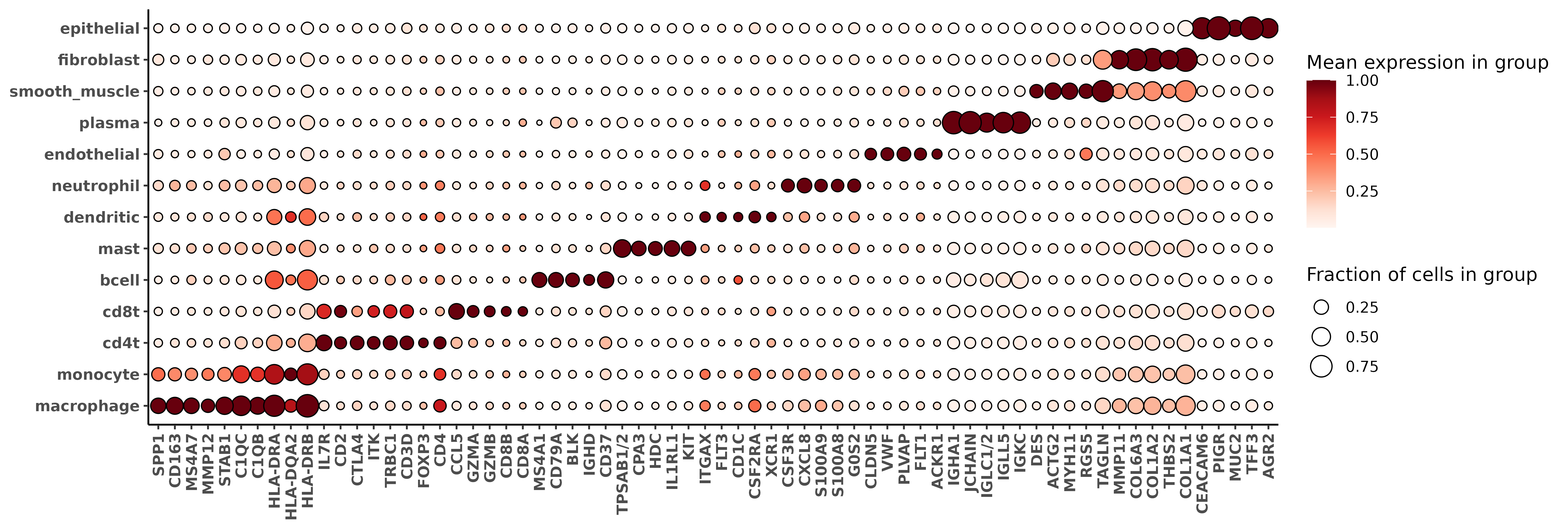
lapply(HieraType::markerslist_immunemajor, "[[", "index_marker")$tcell
[1] "CD3D" "CD3G" "CD3E" "IL7R" "TRBC1" "CD2"
$bcell
[1] "CD19" "MS4A1" "CD79A" "CD79B"
$macrophage
[1] "CD163" "CD68" "MARCO" "CSF1R"
$neutrophil
[1] "MPO" "FCGR3B" "S100A8" "S100A9"
$mast
[1] "KIT" "TPSAB1" "TPSB2" "TPSAB1/2" "CPA3"
$monocyte
[1] "CD14" "FCGR3A" "CCR2" "LYZ"
$dendritic
[1] "ITGAX" "CLEC9A" "FLT3" "XCR1" "CD1C" Here’s a spatial plot of the cell types we’ve called so far. We could stop here, or continue in the same manner for subclassifying any other cell types.
Code
met <- merge(data.table(sem@meta.data)
             ,immune_typing$post_probs$l1[,.(cell_ID, celltype_supervised = celltype_granular)]
             ,by="cell_ID")

colorpal <- c('#F0A0FF','#E0FF66','#C20088','#00998F','#426600'
              , "#4C005C"
              ,'#191919'
              ,'#003380', '#005C31','#94FFB5','#990000','#0075DC','#FFA405')
names(colorpal) <- sort(unique(met[["celltype_supervised"]]))

xyplist_sup <-
  lapply(split(met, by="portion"), function(xx){
    HieraType:::xyplot(cluster_column = "celltype_supervised", metadata = xx
                       , ptsize = 0.1, cls = colorpal
                       #,clusters = c("cd4t", "cd8t", "bcell")
#                       , ptsize = 0.01, cls = colorpal
                       ,plotfirst = c("epithelial", "endothelial", "fibroblast", "smooth_muscle", "plasma")
                       ) + coord_fixed()
  })
xyplot_sup <-
cowplot::plot_grid(plotlist = xyplist_sup,nrow = 1) +
  theme(plot.background = element_rect(fill = 'white',color='white')) +
  cowplot::panel_border(remove=TRUE)
print(xyplot_sup)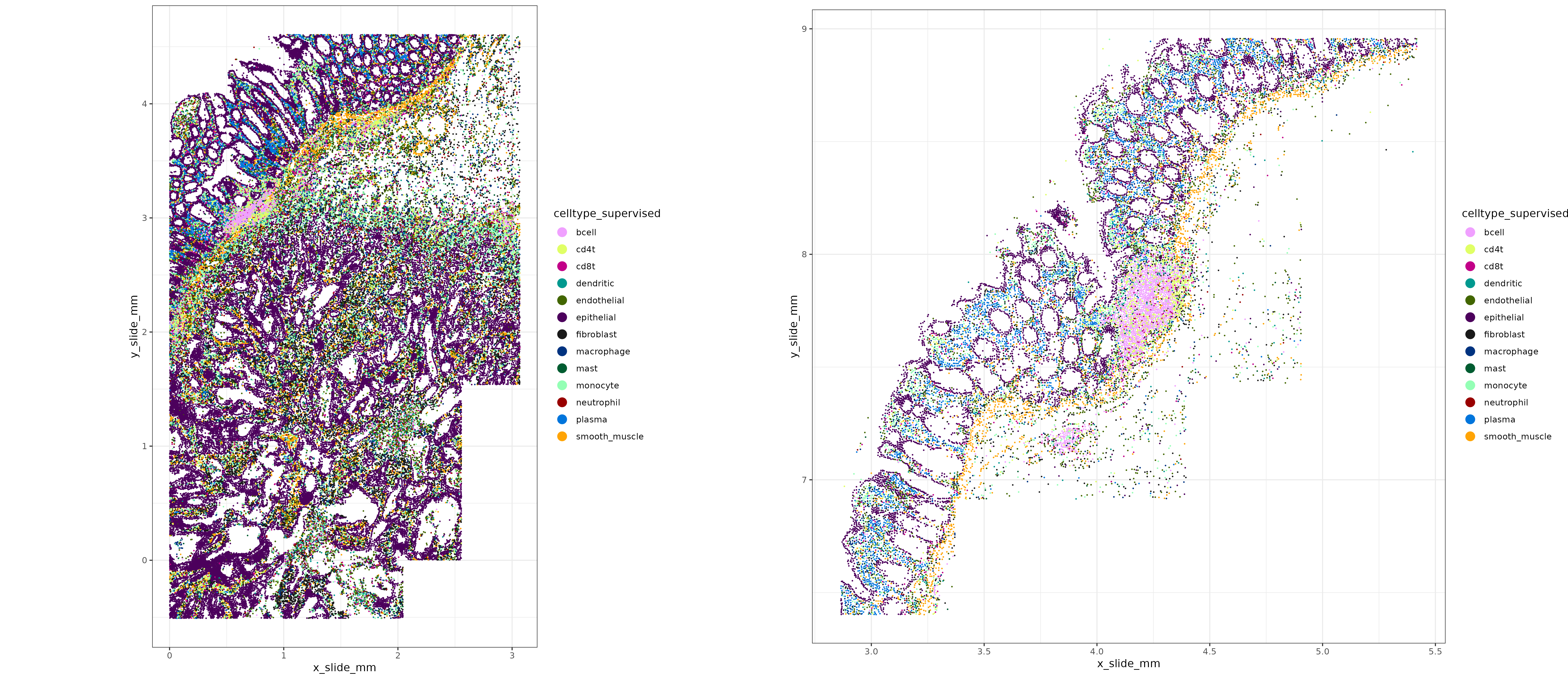
Below, we notice several interesting things about the spatial distribution of cd8t, cd4t, and bcell types. The cd4t cells tend to show higher colocalization with bcells in tertiary lymphoid type structures, while cd8t spatial distribution are more dispersed throughout the tissue. This reflects the role of cd8t cells in seeking out and killing tumor cells, compared to the role of cd4t cells in local antigen presentation.
Code
xyplist_lymph <-
  lapply(split(met, by="portion"), function(xx){
    HieraType:::xyplot(cluster_column = "celltype_supervised", metadata = xx
                       , ptsize = 0.05, cls = colorpal
                       ,clusters = c("cd4t", "cd8t", "bcell")
                       ) + coord_fixed()
  })

lymphplot <-
cowplot::plot_grid(
xyplist_lymph[[1]]  +
  facet_wrap(~celltype_supervised) + ggdark::dark_theme_bw() + theme(text=element_text(size=12,face='bold'))
,xyplist_lymph[[2]]  +
  facet_wrap(~celltype_supervised) + ggdark::dark_theme_bw() + theme(text=element_text(size=12,face='bold'))
,nrow=2
,rel_heights  = c(1.3,1)
)  +
  theme(plot.background = element_rect(fill = 'black',color='black')) +
  cowplot::panel_border(remove=TRUE)


print(lymphplot)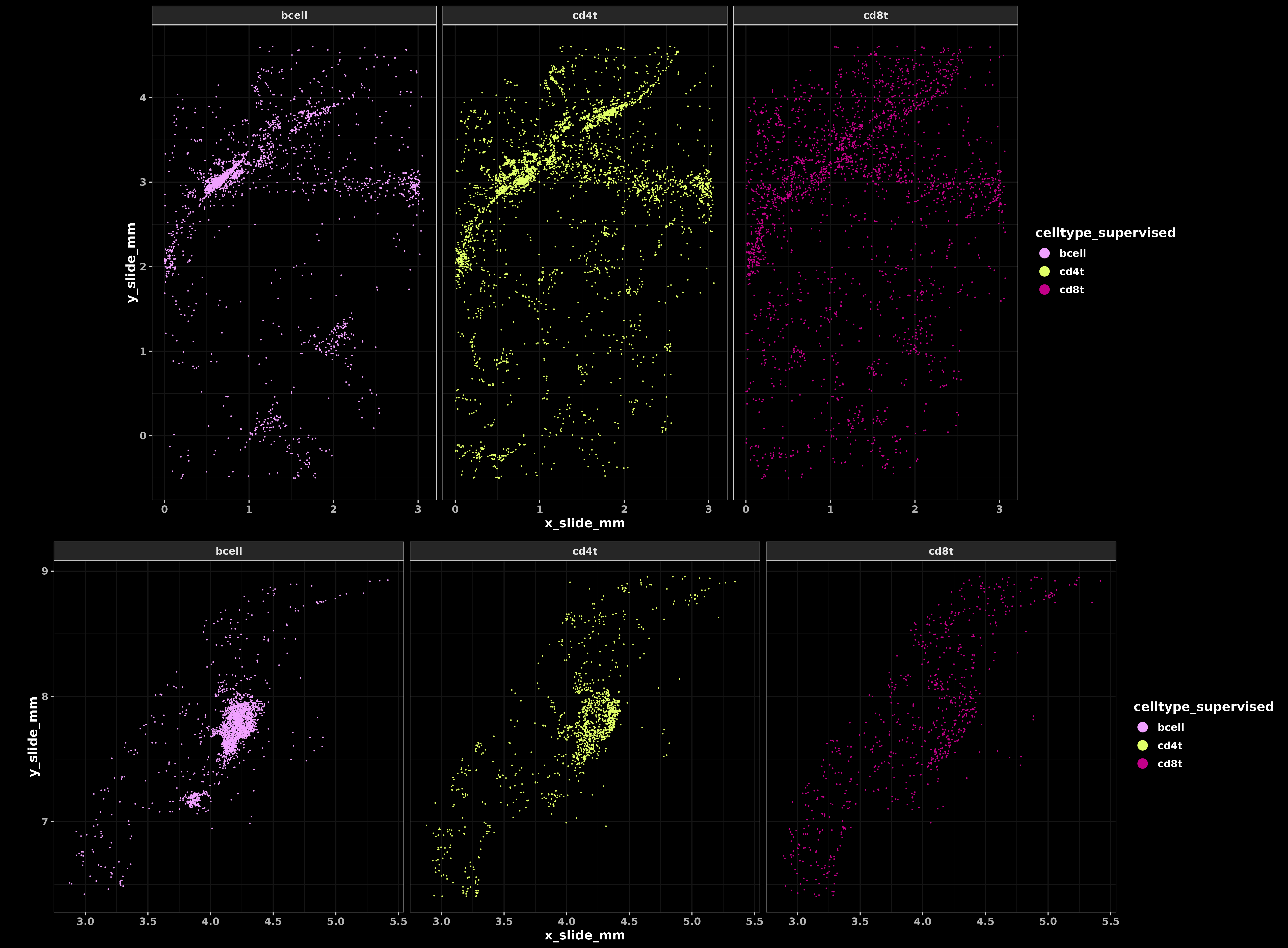
7 Conclusion
We’ve discussed a method for cell typing that uses predefined sets of marker genes to build cell type specific metagene scores, which are probabilistically clustered into cell types.
Using a predefined set of marker genes has several advantages. For one, this allows users to prespecify the network of genes which are expected to have positive covariance within the cell type, and restricts any undesired influence of non-informative or noisy genes. Because no assumption is made regarding the average expression or level of covariance between any pair of genes, we suspect that in some cases this approach may be more flexible and robust in the presence of batch effects or platform effects compared to using pre-trained models, data transfer, or reference profiles which may have been trained using different sample conditions or technologies.
The NNLS regression framework for estimating celltype metagenes allows for improved prediction power by incorporating information from similar cells through an adjacency network. By restricting the direction of the regression coefficients, we’ve implicitly imposed an assumption of positive covariance between these markers within the corresponding cell type class. Sign constraints have been shown to be as effective in some cases as explicit regularization (Slawski and Hein 2013).
We use a mixture of overfitted multivariate gaussian mixture models for probabilistic cell type classification. This approach is effectively a non-parametric mixture model, where we assume that the distribution of metagene scores for each cell type can be approximated by a ‘large-enough’ mixture of multivariate gaussians (Aragam et al. 2020). The simple selection of anchor cells based on score positivity, and ability to fine tune cell typing by controlling behavior of double positivity should allow for easy user control and flexibility.
While we envision the method to be useful for many cell typing applications, there are several caveats and limitations users should keep in mind. One primary assumption is that the user has a sense of the tissue type they are working with and the cell types that are likely to be present. If the user were to run a “tcell typing pipeline” on myeloid cells, they may see unexpected or poor results. Similarly, the “io pipeline” we used in Example 2, may not perform well in a very different tissue type, like brain for example. If we wanted to apply this method to a tissue type like ‘brain’, we may need to generate a new pipeline, with markerslists for brain specific cell types like neurons and oligodendrocytes. For cases where a major cell type exists in a dataset but does not have a markerslists to be modeled, that cell type could manifest as cells which have “low posterior probability” for all of the other cell type classes included in the pipeline.
There are several future improvements for this method we plan to work on. Simultaneous estimation of metagene scores and clustering (perhaps through a regression-based mixture model) might enhance the power of metagene scores and classification by optimizing the cell allocations to the correct cluster simultaneously during model-fitting. Exploring other frameworks outside of NNLS regression could potentially capture more flexible model structures with interaction and non-linearity.
The ability or freedom to learn additional marker genes from the data, and an extension to a semi-supervised framework where cell types where marker genes are unknown a priori would also be useful.
We’ve implemented the tools presented here in the R package HieraType.
8 Quick summary of package functions used in this post
Below we call out a short list of HieraType package functions which were used throughout this post. Please see the examples throughout the rest of this document for more context on their usage.
Model Fitting and Clustering
make_markerlist()- Used to create a custom list of cell type markers.make_pipeline()- Used to create a pipeline, or recipe for hierarchical cell typing.run_pipeline()- Used to run a hierarchical cell typing pipeline.fit_metagene_scores()- This function fits cell type metagene scores. Called as a standalone function or automatically withinrun_pipeline,cluster_metagenes()- This function clusters cell type metagene scores using overfitted-gaussian mixture models. Also called withinrun_pipeline.
Plotting and Diagnostics
xyplot()- A utility function for plotting cell types in x/y space.metagene_pairsplot()- Plot pairwise distributions of metagene scores.metagene_coefficients_plot()- Plot for which genes contribute most to cell type metagene scores.marker_threshold_plot()- Model diagnostics plot, show specific marker genes and the proportion of cells that express them by cluster, for increasing posterior probability thresholds.clusterwise_foldchange_metrics()- Computes the fold change, average expression, proportion of cells with at least 1 count for each gene and each cluster. This is the data used as input to a marker gene heatmap.marker_heatmap()- Makes a bubble-style heatmap plot (clusters x marker genes) showing the proportion of cells with at least one count (bubble size) and relative average expression (bubble color). Easy to add and control the genes shown in the heatmap, and can specify a fixed order for comparing multiple heatmaps.
References
Aragam, Bryon, Chen Dan, Eric P. Xing, and Pradeep Ravikumar. 2020. “Identifiability of nonparametric mixture models and Bayes optimal clustering.” The Annals of Statistics 48 (4): 2277–2302. https://doi.org/10.1214/19-AOS1887.
Sigg, Christian D., and Joachim M. Buhmann. 2008. “Expectation-Maximization for Sparse and Non-Negative PCA.” In Proceedings of the 25th International Conference on Machine Learning, 960–67. ICML ’08. New York, NY, USA: Association for Computing Machinery. https://doi.org/10.1145/1390156.1390277.
Slawski, Martin, and Matthias Hein. 2013. “Non-negative least squares for high-dimensional linear models: Consistency and sparse recovery without regularization.” Electronic Journal of Statistics 7 (none): 3004–56. https://doi.org/10.1214/13-EJS868.