1 Introduction

Annotated Data, AnnData, is a popular data structure for exploring and analyzing high-plex single-cell data, including spatial transcription data. There are quite a few open-sourced single-cell analysis tools in python, e.g. scanpy and squidpy, as well as interactive viewers, e.g. Cirrocumulus and CELLxGENE viewers, using this data structure. Converting CosMx™ spatial data sets into anndata data structure allows non-coders to easily share the light-weighted data object, visualize and explore the processed data in an interactive way.

This post describes how to create anndata object (.h5ad) from either a post-analysis Seurat object or basic data files exported from AtoMx™ Spatial Informatics Portal (SIP). We hope this post would facilitate seamless integration of CosMx™ spatial data sets into Python-based single-cell analysis workflows.

Section 2 Creating an anndata object in .h5ad format from post-analysis Seurat object exported by AtoMx™ SIP
Section 3 Visualize the post-analysis .h5ad object in an interactive viewer
Section 4 Creating per-sample anndata object from basic data files in Python for python-based single-cell analysis

Like other items in our CosMx Analysis Scratch Space, the usual caveats and license applies.

2 Creating an `anndata` object from post-analysis `Seurat` object exported by AtoMx™ SIP

AtoMx™ SIP can export a CosMx™ Spatial Molecular Imager (SMI) study into Seurat data objects for direct usage in R. Here we first work in R to open, visualize, and make minor adjustments to the object. We then export it into a .h5ad file for usage in Python tools.

The Seurat object used in this section is made from the CosMx™ mouse brain public data set and assembled in the structure used by the Technology Access Program (TAP); similar outputs are available from the AtoMx™ SIP. To download raw data for this dataset, go here. For more details on its data structure, please refer to earlier post on Visualizing spatial data with Seurat.

Important

All the code in this section 2 is in R.

Note

Many of the below functions require that you are working with Seurat v5 and may not work in earlier versions. Additionally, if you are exporting a Seurat object from AtoMx (v1.3+), be sure to export the Seurat object with polygon coordinates and transcripts included to access all of the functionality below.

2.1 Explore post-analysis `Seurat` object and add in custom cell meta data

Setup R

library(Seurat)
library(SeuratObject)
library(SeuratDisk)
library(ggplot2)

# load existing seurat object
seu.obj <- readRDS("seurat_object.Rds")

The post-analysis Seurat object exported from AtoMx™ SIP should contain

expression matrices for various feature types, like RNA, RNA_normalized, negprobes and falsecodes;
dimension reduction results, like pca and umap;
results for graphs, like snn and nn.

You can visualize which results are included by running names(seu.obj). The exact names of the results stored in your post-analysis Seurat object might be slightly different from what are included in the particular example here. Please adjust the code accordingly.

You can also add in any new cell metadata if desired. For illustration, the code below adds a new column with unique ID for each FOV.

# add a new column for unique ID of each FOV
fovNames <- seu.obj@meta.data[, c('slide_ID_numeric', 'fov')]
fovNames[['fov_names']] <- paste0('fov_', fovNames[['slide_ID_numeric']], 
                            '_', fovNames[['fov']])
fovNames <- setNames(fovNames[['fov_names']], 
                     nm = rownames(fovNames))

seu.obj <- Seurat::AddMetaData(seu.obj, 
                               metadata = fovNames, 
                               col.name = "fov_names")

2.2 Prepare spatial coordinates and visualize

AtoMx™ SIP stores the per-slide cell segmentation information as separate SeuratObject::FOV objects in the images slot. You can get the slide names by running names(seu.obj@images) in R.

The example dataset used in this section has two tissue slides in one study and each slide is in its own spatial coordinate space and thus may have xy overlapping between the slides.

2.2.1 Case 1: 1 slide per `anndata` object

When a per-slide anndata object is preferred, one should split the Seurat object by the slide name first before cleaning it up in section 2.3. The code below is for generating one anndata object per tissue slide and the resulting data is used in later sections.

# extract the segmentation to separate variable
imgList <- seu.obj@images

# remove segmentation in current seurat object before split
for (slideName in names(imgList)){
  seu.obj[[slideName]] <- NULL
}

# split Seurat object by slide name which is stored under "Run_Tissue_name" column of cell meta.data. 
objList <- Seurat::SplitObject(seu.obj, split.by = "Run_Tissue_name")

# You can add the segmentation back for each per-slide object 
for (eachSlide in names(objList)){
  # standard names used in `images` slot
  slideName <- gsub("\\W|_", ".", eachSlide)
  # add the `SeuratObject::FOV` object for current slide alone
  objList[[eachSlide]][[slideName]] <- imgList[[slideName]]
}

We would focus on the first slide for this section.

# keep data for only the 1st section for analysis in later section
eachSlide <- names(objList)[1]
slideName <- gsub("\\W|_", ".", eachSlide)
seu.obj1 <- objList[[eachSlide]]

# extract spatial coordinates of each cell for the chosen slide
spatial_coords <- seu.obj1[[slideName]]$centroids@coords
rownames(spatial_coords) <- seu.obj1[[slideName]]$centroids@cells

Let’s visualize the current cell segmentation colored by cell types and the molecular positions of a few selected genes. For more visualization tricks using Seurat, please refer to earlier post and Seurat’s vignette on image-based spatial data analysis.

# specify to show cell boundary 
SeuratObject::DefaultBoundary(seu.obj1[[slideName]]) <- "segmentation"

Seurat::ImageDimPlot(object = seu.obj1, 
                     fov = slideName, 
                     
                     # column name of cell type in meta.data
                     group.by = "nb_clus_final", 
                     
                     # specify which molecules to plot
                     molecules = c("Slc17a7", "Gad1", "Plp1"), 
                     mols.size = 1.5, 
                     
                     # fixed aspect ratio and flip xy in plotting
                     coord.fixed = TRUE, flip_xy = TRUE)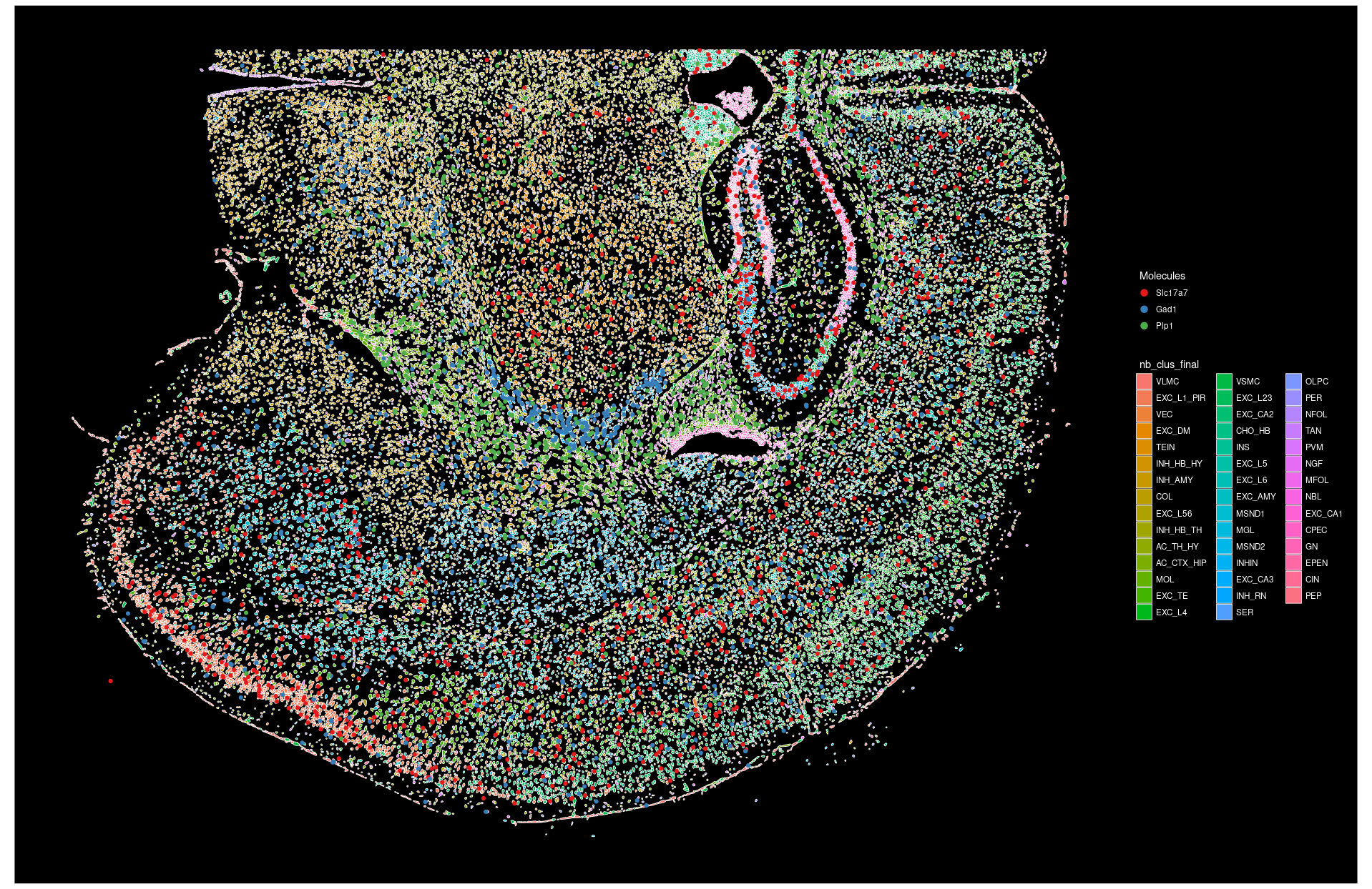

You can zoom in to view a subset of cells by specifying which cells to plots.

# change idents to "fov" for cell selection
# note: "fov" here is a column in cell meta.data instead of the `SeuratObject::FOV` object. 
SeuratObject::Idents(seu.obj1) <- "fov"

Seurat::ImageDimPlot(object = seu.obj1, 
                     fov = slideName, 
                     
                     # column name of cell type in meta.data
                     group.by = "nb_clus_final", 
                     
                     # a vector of chosen cells, plot cells in chosen fovs
                     cells = SeuratObject::WhichCells(
                       seu.obj1, idents = c(72:74, 90:92, 97:99, 114:116)), 
                     
                     # crop the plots to area with cells only
                     crop = TRUE, 
                     
                     # fixed aspect ratio and flip xy in plotting
                     coord.fixed = TRUE, flip_xy = TRUE)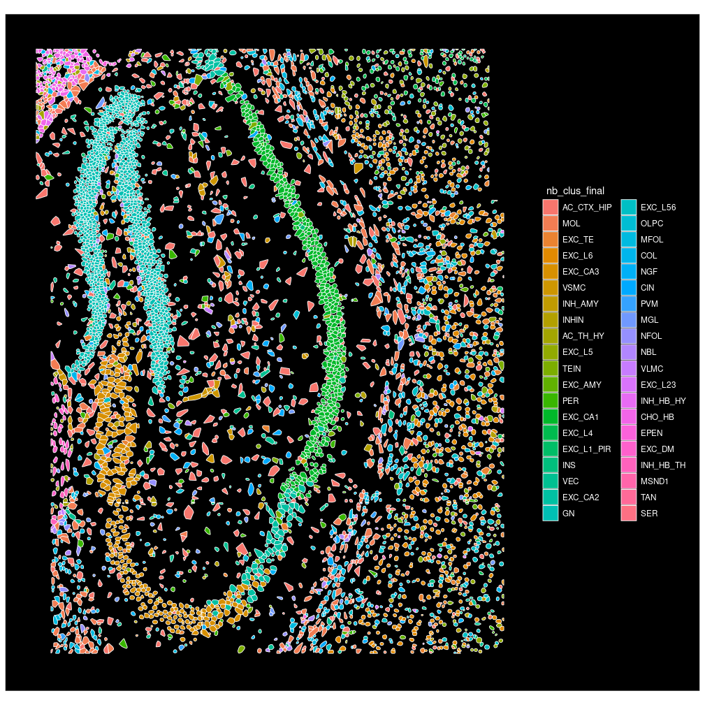

2.2.2 Case 2: multi-slide per `anndata` object

Since AtoMx™ SIP keeps the spatial coordinates of each slide in their own spatial coordinate space, one would need to arrange the spatial coordinates of multiple sample sections to avoid overlap in XY space when exporting multiple slides in same study-level anndata object. The example code below would arrange all slides along Y axis with some spacing between the slides.

# extract the segmentation to separate variable
imgList <- seu.obj@images

# arrange slides along Y axis, add in spacer which is 0.2x of previous slide's coordinate span in Y direction
spacerFactor <- 0.2
global_y_offset <- 0 

spatial_coords <- lapply(imgList, function(img){
  # coordinates of query slide
  eachCoord <- img$centroids@coords
  rownames(eachCoord) <- img$centroids@cells
  
  # align to lower left corner
  ori_offsets <- apply(eachCoord, 2, min)
  eachCoord <- sweep(eachCoord, 2, ori_offsets, "-")
  
  # span in y direction
  y_span <- diff(range(eachCoord[, 2]))

  # add spacer in y direction 
  eachCoord[, 2] <- eachCoord[, 2] + global_y_offset
  
  # update global offset for next slide
  global_y_offset <<- global_y_offset + y_span*(1+spacerFactor)
  
  return(eachCoord)
})
spatial_coords <- do.call(rbind, spatial_coords)  

# use the study-level Seurat object for downstream
seu.obj1 <- seu.obj

# prefix for file name
slideName <- "StudyLevel"

Let’s visualize the coordinates of all cells after slide arrangement.

# add in cell type for color
plotData <- cbind(seu.obj1[["nb_clus_final"]], 
                  spatial_coords[colnames(seu.obj1), ])

ggplot2::ggplot(plotData, 
                # flip xy to be consistent with earlier plots
                ggplot2::aes(x = y, y = x, color = as.factor(nb_clus_final))) +
  ggplot2::geom_point(size = 0.1)+
  ggplot2::coord_fixed()+
  Seurat::NoLegend()+
  Seurat::DarkTheme()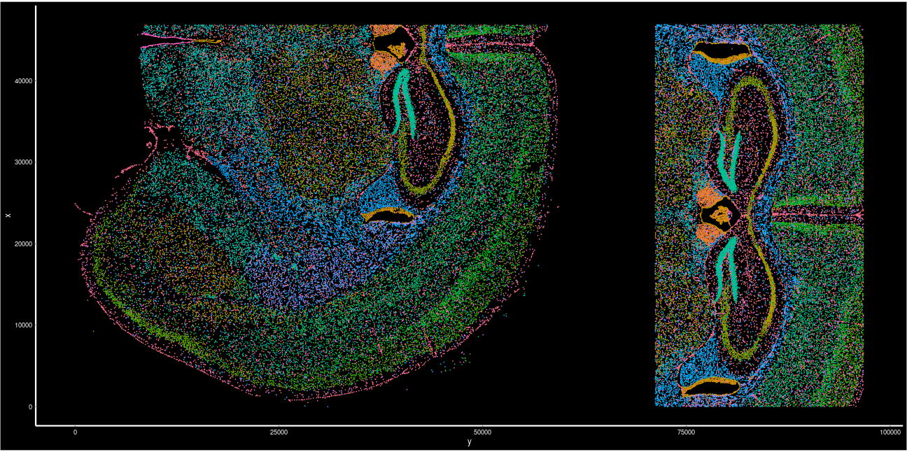

2.3 Clean up to keep only necessary data

Next, we would further clean up the Seurat object (single-slide object from Case 1 in section 2.2.1 or full-study-level object from Case 2 in section 2.2.2) by trimming it down to contain only the data of interested.

Typically, one would keep the raw data counts from RNA assay (this example dataset uses Nanostring as assay name for RNA), cell embedding for umap (standard AtoMx exported object uses approximateumap as name for umap). We would also store the spatial coordinates of each cell as the cell embedding in a dimension reduction object called spatial.

# clean up seurat object to only necessary data 
seu.obj2 <- Seurat::DietSeurat(
  seu.obj1, 
  
  # subset of assays to keep, standard AtoMx object uses "RNA" assay
  # of note, AtoMx stores normalized RNA counts in separate "RNA_normalized" assay
  assays = "Nanostring",
  
  # keep raw counts stored in "counts" layer
  # use "data" or "scale.data" if prefer to keep normalized counts before or after scaling
  layers = "counts", 
  
  # dimension reduction to keep, standard AtoMx object uses "approximateumap"
  dimreducs = "umap")

# clear the `images` slot
allImgs <- names(seu.obj1@images)
for (img in allImgs){
  seu.obj2[[img]] <- NULL
}

# add in spatial coordinates for current slide or study as a new dimension reduction
colnames(spatial_coords) <- paste0("SPATIAL_", seq_len(ncol(spatial_coords)))
seu.obj2[["spatial"]] <- Seurat::CreateDimReducObject(
  embeddings = spatial_coords, 
  key = "SPATIAL_", 
  # standard AtoMx object use "RNA" assay
  assay = "Nanostring")

2.4 Converting to `h5ad` format via `h5Seurat`

Lastly, we would export the cleaned Seurat object into h5Seurat format and then further convert it into h5ad format using SeuratDisk::Convert function.

# export as "h5Seurat" object in your current working directory
SeuratDisk::SaveH5Seurat(seu.obj2, 
                         filename = paste0(slideName, "_subset.h5Seurat"))

Creating h5Seurat file for version 3.1.5.9900 Adding counts for Nanostring Adding data for Nanostring No variable features found for Nanostring No feature-level metadata found for Nanostring Adding cell embeddings for umap No loadings for umap No projected loadings for umap No standard deviations for umap No JackStraw data for umap Adding cell embeddings for spatial No loadings for spatial No projected loadings for spatial No standard deviations for spatial No JackStraw data for spatial

# convert to h5ad format
SeuratDisk::Convert(paste0(slideName, "_subset.h5Seurat"), 
                    dest = "h5ad")

Validating h5Seurat file Adding data from Nanostring as X Adding counts from Nanostring as raw Transfering meta.data to obs Adding dimensional reduction information for spatial Adding dimensional reduction information for umap

3 Visualize the post-analysis `.h5ad` object in an interactive viewer

The resulting anndata object in .h5ad format could be visualized by various open-sourced interactive viewers. One such viewer would be Cirrocumulus viewer.

For a quick start, one can install the viewer in terminal via pip.

Terminal

pip install cirrocumulus

Create virtual environment for viewer

It’s recommended to create separate virtual environment for viewer. The current released version of cirrocumulus viewer is in version 1.1.57 and has package dependencies as listed below.

Python >= 3.9.7 and Python <= 3.9.18
pandas >= 1.3.4 and pandas <= 2.1.0
anndata >= 0.9.1 and <= 0.10.2

One can create a new environment with specific version of packages for this viewer using various package managers in terminal. One of such managers that people often use is conda and below is an example code.

Terminal

conda create --name myenv python==3.9.18 pandas==2.1.0 anndata==0.10.2

To activate an existing environment, one should pass the name of environment to conda activate function.

Terminal

conda activate myenv

To launch the viewer for the .h5ad object of interest, one can simply run

Terminal

cirro launch <path_to_dataset_file.h5ad>

The cirrocumulus viewer allows user to

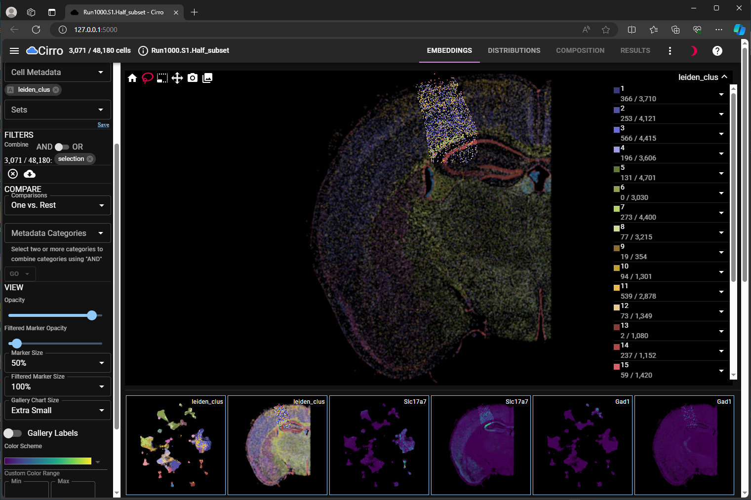
view multiple cell embeddings (umap and spatial) side-by-side for both cell metadata and gene expression (Figure 1, Dual Embedding View);
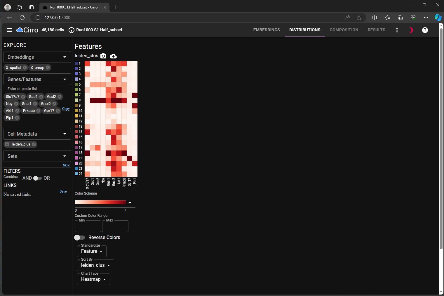
use lasso tool to subset cells of interest in the embedding space (Figure 2, Lasso-in-Space);
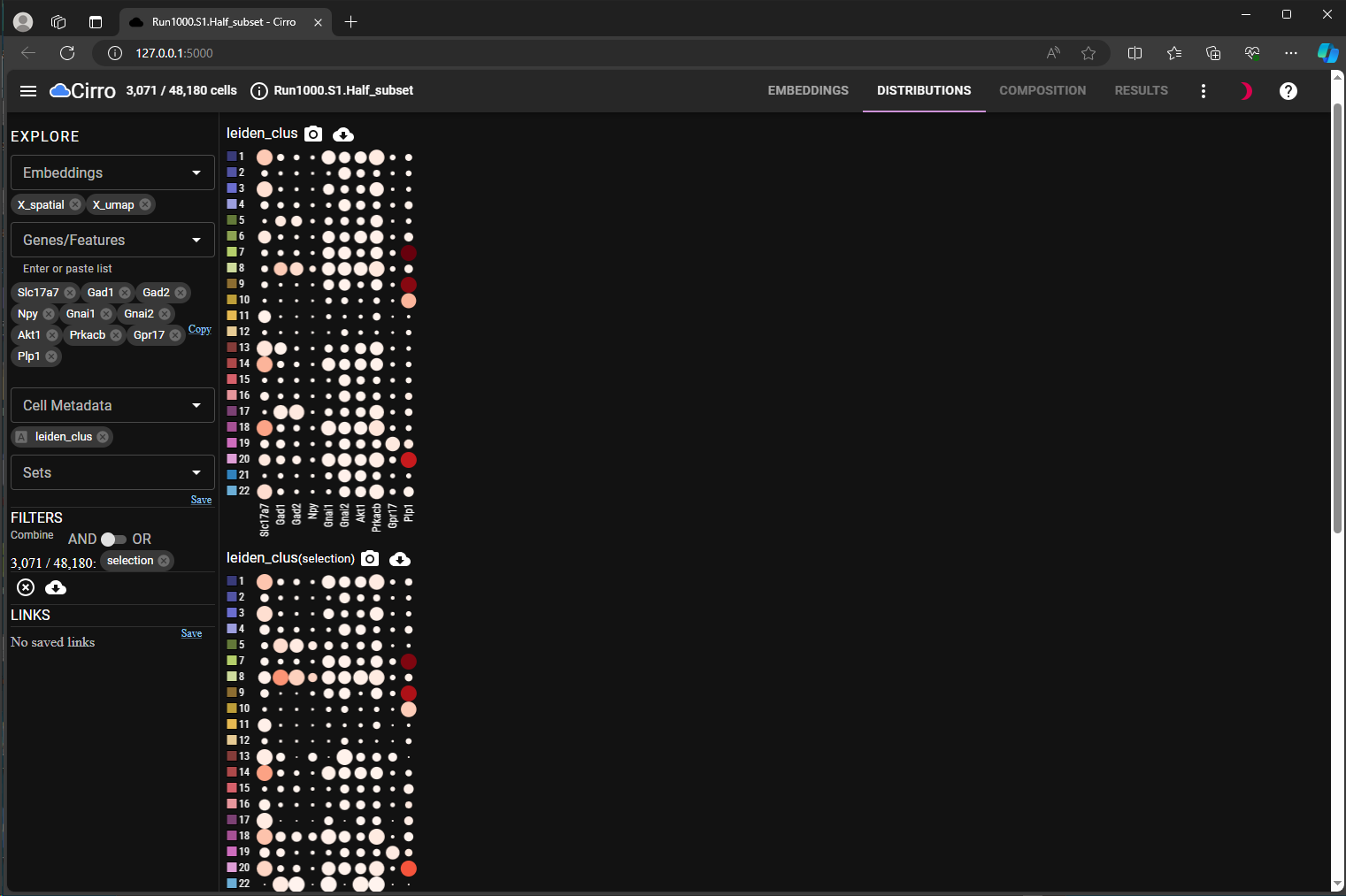
explore how the gene expression changes between different selections (Figure 3, Marker Heatmap for all cells vs. Figure 4, Dot Plots for Subsets).

For more information, please refer to the documentation of cirrocumulus package

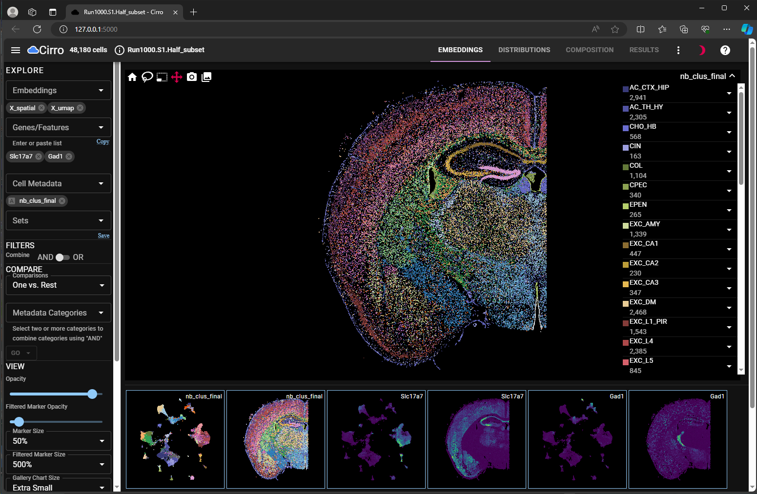
Figure 1: The dual-embedding views of `umap` and `spatial` for chosen cell meta data and gene expression level.

Figure 2: Use lasso tool to select cells in `spatial` embedding. Chosen cells are shown in solid colors.

Figure 3: Heatmap of selected gene expression across ‘leiden_clus’ of all cells.

Figure 4: Dot plots of chosen gene expression for all cells (top) vs. cells within lasso selection (bottom) in Figure 2 tab.

4 Creating per-sample `anndata` object from basic data files in `Python` for python-based single-cell analysis

For python lovers, it may be desired to create anndata object from scratch and then feed it into python-based single-cell analysis tools, like scanpy and squidpy.

In this section, we start from the basic data files (in .csv format) exported from AtoMx™ SIP. For an example public dataset that you can download, go here.

AtoMx™ SIP splits and organizes the basic data files by tissue slides during export. Thus, unlike the Seurat object of the mouse brain dataset used in earlier section 2, the basic data files used for this section 4 contain information for one single slide of pancreas sample. The ReadMe associated with this example data set on pancreas shows the data structures of each file used in this section.

Important

All the code in this section 4 is in Python.

Setup Python

import os
import re
import numpy as np
import pandas as pd
import anndata as ad
from scipy.sparse import csr_matrix

# path to folder of downloaded basic data files
dataDir = "Pancreas-CosMx-WTx-FlatFiles"

Firstly, we would load the raw expression matrix and assign row names for cell in same naming pattern as the ones in cell meta data file. For demonstration purpose, we would focus on just the RNA probes and remove all the control probes.

# read in cell expression file
df = pd.read_csv(os.path.join(dataDir, 'Pancreas_exprMat_file.csv'))

# create row names for "cell" in same format as what's used in cell metadata file
# the new cell_ID has pattern as 'c_[slideID]_[cell_ID]', where slideID = 1 in this example dataset
df["new_cell_ID"] =  df.apply(lambda row: f"c_1_{row.fov}_{row.cell_ID}", axis = 1)
df.set_index("new_cell_ID", inplace=True)

# drop annotation columns
df.drop(columns=["fov", "cell_ID"], inplace=True)

# focus on RNA probes while drop control probes
dummy=re.compile(r'Negative|SystemControl', flags=re.IGNORECASE)
chosen_probes = [col for col in list(df.columns) if not dummy.search(col)]

# "cell" names for ordering downstream
chosen_cells = df.index

# convert to a sparse matrix
raw = csr_matrix(df[chosen_probes].astype(pd.SparseDtype("float64",0)).sparse.to_coo())

# delete unused variable to free up memory
del df

Next, we would read in the cell meta data and extract the spatial coordinates of each cell. Based on the ReadMe of these data files, we can know this data set has pixel size of 0.12028 µm per pixel. For illustration, we also convert the pixel coordinates to µm here.

# read in cell meta data file
cell_meta = pd.read_csv(os.path.join(dataDir, 'Pancreas_metadata_file.csv'))

# use "cell" column as row names to match with raw expression matrix
# for convenience, the "cell" column is kept with the meta data
cell_meta.set_index("cell", inplace=True, drop = False)

# extract spatial coordinates of cells, use the global coordinates
coords = cell_meta[["CenterX_global_px","CenterY_global_px"]]

# use "x" and "y" as column names
coords = coords.rename(columns={"CenterX_global_px":"x", 
                                "CenterY_global_px": "y"})

# reorder cells to be in same row order as raw expression matrix
coords = coords.reindex(index = chosen_cells)

# convert px coordinates to micrometer 
pixel_size = 0.12028
coords = coords.mul(pixel_size)

Now, we are ready to create the anndata object using anndata.AnnData() python function. We would add the spatial coordinates as an annotation array stored in obsm slot.

adata = ad.AnnData(
    X = raw, 
    obs = cell_meta, 
    # row names should be the same as gene names
    var = pd.DataFrame(
        list(chosen_probes), 
        columns = ["gene"],
        index = chosen_probes))
                   
# add spatial coordinates 
adata.obsm['spatial'] = coords.to_numpy()

# you can add name of slide or original file as one of unstructured annotation
adata.uns['name'] = "Pancreas"

# convert string columns to categorical data in `obs`
adata.strings_to_categoricals()

Add additional embedding

You can add additional embedding if exists. The code below assumes you have a new embedding for umap stored in umap.csv file as a data frame with rows in same order as the cell expression file.

adata.obsm['umap'] = pd.read_csv(os.path.join(dataDir, 'umap.csv')).to_numpy()

In some case, one may want to convert a meta data column with numeric values (like numeric ID for cell clusters) to categorical data, you can do this as shown below.

# for illustration, we would convert the "fov" column here
columnName = "fov"
adata.obs[columnName] = pd.Categorical(adata.obs[columnName].astype(str))

You can also specific color for each categorical value via a dictionary. Most viewers based on anndata data structure would be able to recognize the color information stored under [cell_meta_name]_colors when displaying the corresponding categorical cell meta data.

# use random colors for illustration here
import random

colors_dict = {}
for catVal in adata.obs[columnName].cat.categories:
    # random RGB value
    [r, g, b] = [random.randint(0, 255) for _ in range(3)]
    # convert to hex format
    colors_dict[catVal] = "#{:02x}{:02x}{:02x}".format(r, g, b)

# add to `uns` slot
colorName = "_".join((columnName, "colors"))
adata.uns[colorName] = [colors_dict[k] for k in adata.obs[columnName].cat.categories]

At this point, we have a anndata object that could be exported to .h5ad file format and pass to other python-based single-cell analysis tools, like scanpy and squidpy.

Export as .h5ad file

adata.write(os.path.join(dataDir, "Pancreas_basic.h5ad"), compression="gzip")

Load existing .h5ad file

import scanpy as sc
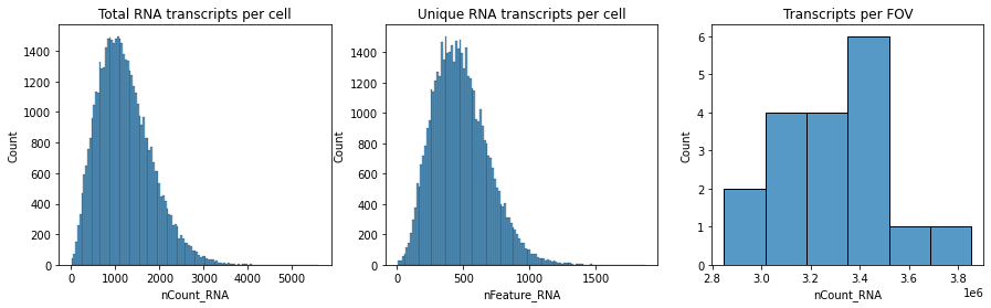
adata = sc.read(os.path.join(dataDir, "Pancreas_basic.h5ad"))

Let’s visualize the distribution of some cell meta data saved in this anndata object.

import matplotlib.pyplot as plt
import seaborn as sns

# plot transcripts distribution
fig, axs = plt.subplots(1, 3, figsize=(15, 4))

axs[0].set_title("Total RNA transcripts per cell")
sns.histplot(
    adata.obs["nCount_RNA"],
    kde=False,
    ax=axs[0],
)

axs[1].set_title("Unique RNA transcripts per cell")
sns.histplot(
    adata.obs["nFeature_RNA"],
    kde=False,
    ax=axs[1],
)

axs[2].set_title("Transcripts per FOV")
sns.histplot(
    adata.obs.groupby("fov").sum()["nCount_RNA"],
    kde=False,
    ax=axs[2],
)

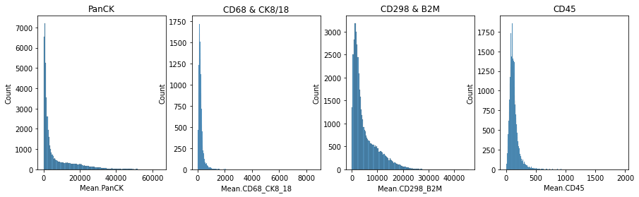
# plot immune intensity distribution
fig, axs = plt.subplots(1, 4, figsize=(15, 4))

axs[0].set_title("PanCK")
sns.histplot(
    adata.obs["Mean.PanCK"],
    kde=False,
    ax=axs[0],
)

axs[1].set_title("CD68 & CK8/18")
sns.histplot(
    adata.obs["Mean.CD68_CK8_18"],
    kde=False,
    ax=axs[1],
)

axs[2].set_title("CD298 & B2M")
sns.histplot(
    adata.obs["Mean.CD298_B2M"],
    kde=False,
    ax=axs[2],
)

axs[3].set_title("CD45")
sns.histplot(
    adata.obs["Mean.CD45"],
    kde=False,
    ax=axs[3],
)

For more details on how to analyze spatial data sets using python tools, please refer to the tutorials provided by scanpy and squidpy packages.

5 Conclusions

In summary, anndata serves as a versatile data structure in Python-based single-cell analysis. This post outlines how to create anndata object in .h5ad file format from AtoMx™ SIP exported results, which are either a post-analysis Seurat object or basic data files in .csv format. The conversion of AtoMx™ SIP exported results into .h5ad file would facilitate seamless integration into Python-based single-cell analysis workflows. Leveraging Python libraries like scanpy and squidpy, as well as interactive viewers such as Cirrocumulus and CELLxGENE viewers, researchers can share the lightweight data objects, visualize processed data, and explore them in more avenues.

1 Introduction

2 Creating an anndata object from post-analysis Seurat object exported by AtoMx™ SIP

2.1 Explore post-analysis Seurat object and add in custom cell meta data

2.2 Prepare spatial coordinates and visualize

2.2.1 Case 1: 1 slide per anndata object

2.2.2 Case 2: multi-slide per anndata object

2.3 Clean up to keep only necessary data

2.4 Converting to h5ad format via h5Seurat

3 Visualize the post-analysis .h5ad object in an interactive viewer

4 Creating per-sample anndata object from basic data files in Python for python-based single-cell analysis

5 Conclusions

2 Creating an `anndata` object from post-analysis `Seurat` object exported by AtoMx™ SIP

2.1 Explore post-analysis `Seurat` object and add in custom cell meta data

2.2.1 Case 1: 1 slide per `anndata` object

2.2.2 Case 2: multi-slide per `anndata` object

2.4 Converting to `h5ad` format via `h5Seurat`

3 Visualize the post-analysis `.h5ad` object in an interactive viewer

4 Creating per-sample `anndata` object from basic data files in `Python` for python-based single-cell analysis